Skip to article frontmatterSkip to article content
Site not loading correctly?

This may be due to an incorrect BASE_URL configuration. See the MyST Documentation for reference.

2.2: Orthonormal bases in ℝ²

In Chapter 1.4, we wrote vectors as linear combinations of the standard basis vectors. Could we use a different pair of directions? In this section, we’ll see why perpendicular unit vectors make this especially convenient.


The standard basis

Recall the standard basis vectors from Chapter 1.4:

e⃗1=[10],e⃗2=[01].\vec e_1= \begin{bmatrix} 1\\ 0 \end{bmatrix}, \qquad \vec e_2= \begin{bmatrix} 0\\ 1 \end{bmatrix}.

Every vector in R2\mathbb R^2 is a linear combination of these two vectors. Its entries give the coefficients.
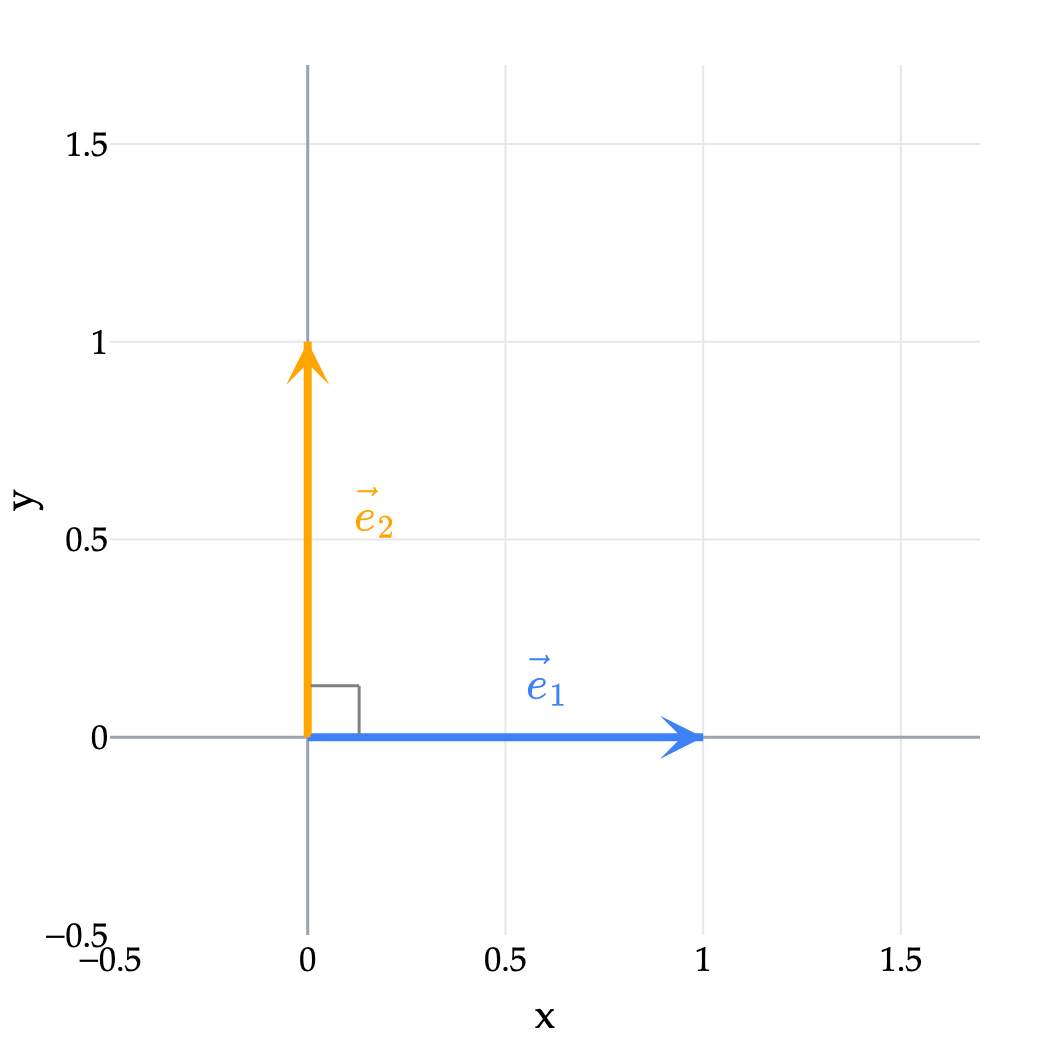
Image produced in Jupyter

The standard basis vectors in R2\mathbb{R}^2.

For example,

[57]=[50]+[07]=5[10]+7[01]=5e⃗1+7e⃗2.\begin{bmatrix} 5\\ 7 \end{bmatrix} = \begin{bmatrix} 5\\ 0 \end{bmatrix} + \begin{bmatrix} 0\\ 7 \end{bmatrix} = 5 \begin{bmatrix} 1\\ 0 \end{bmatrix} + 7 \begin{bmatrix} 0\\ 1 \end{bmatrix} = 5\vec e_1+7\vec e_2.

To do geometry in R2\mathbb{R}^2, it is useful to consider other such pairs of vectors. The key properties of (e⃗1,e⃗2)(\vec e_1,\vec e_2) are:

  1. length one,

  2. orthogonal to each other.

These two properties will let us find coefficients using dot products, even when the directions are tilted.

Recall from Chapter 1.5 that a unit vector has length one. We can turn any nonzero vector w⃗\vec w into a unit vector by dividing by its length: w⃗/∥w⃗∥\vec w/\lVert\vec w\rVert.


Building an orthonormal basis

First, let’s check the lengths of two vectors.

The vector

[4535]\begin{bmatrix} \frac45\\[2pt] \frac35 \end{bmatrix}

has length one since

(45)2+(35)2=1625+925=1.\sqrt{\left(\frac45\right)^2+\left(\frac35\right)^2} = \sqrt{\frac{16}{25}+\frac{9}{25}} = 1.

A unit vector can point in a different direction. For example, the vector

[12−12]\begin{bmatrix} \frac{1}{\sqrt{2}}\\[2pt] -\frac{1}{\sqrt{2}} \end{bmatrix}

has length one since

(12)2+(−12)2=12+12=1.\sqrt{ \left(\frac{1}{\sqrt{2}}\right)^2+ \left(-\frac{1}{\sqrt{2}}\right)^2 } = \sqrt{\frac12+\frac12} = 1.
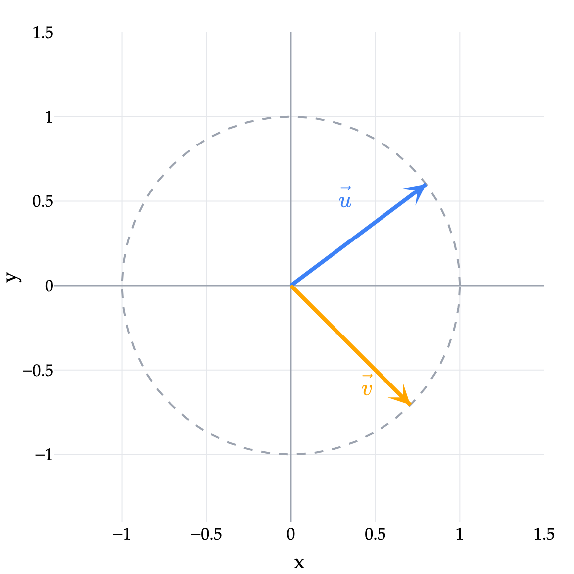
Image produced in Jupyter

Examples of unit vectors in R2\mathbb{R}^2: u⃗=[4/53/5]\vec u=\begin{bmatrix}4/5\\3/5\end{bmatrix} and v⃗=[1/2−1/2]\vec v=\begin{bmatrix}1/\sqrt{2}\\-1/\sqrt{2}\end{bmatrix}. These vectors both have length one, but they are not orthogonal to each other.

To make an orthonormal basis, we need two unit vectors that are also perpendicular. Let

u⃗1=[4535],u⃗2=[−3545].\vec u_1= \begin{bmatrix} \frac45\\[2pt] \frac35 \end{bmatrix}, \qquad \vec u_2= \begin{bmatrix} -\frac35\\[2pt] \frac45 \end{bmatrix}.

Both vectors have length one, and their dot product is

u⃗1⋅u⃗2=45(−35)+35(45)=0.\vec u_1\cdot\vec u_2=\frac45\left(-\frac35\right)+\frac35\left(\frac45\right)=0.

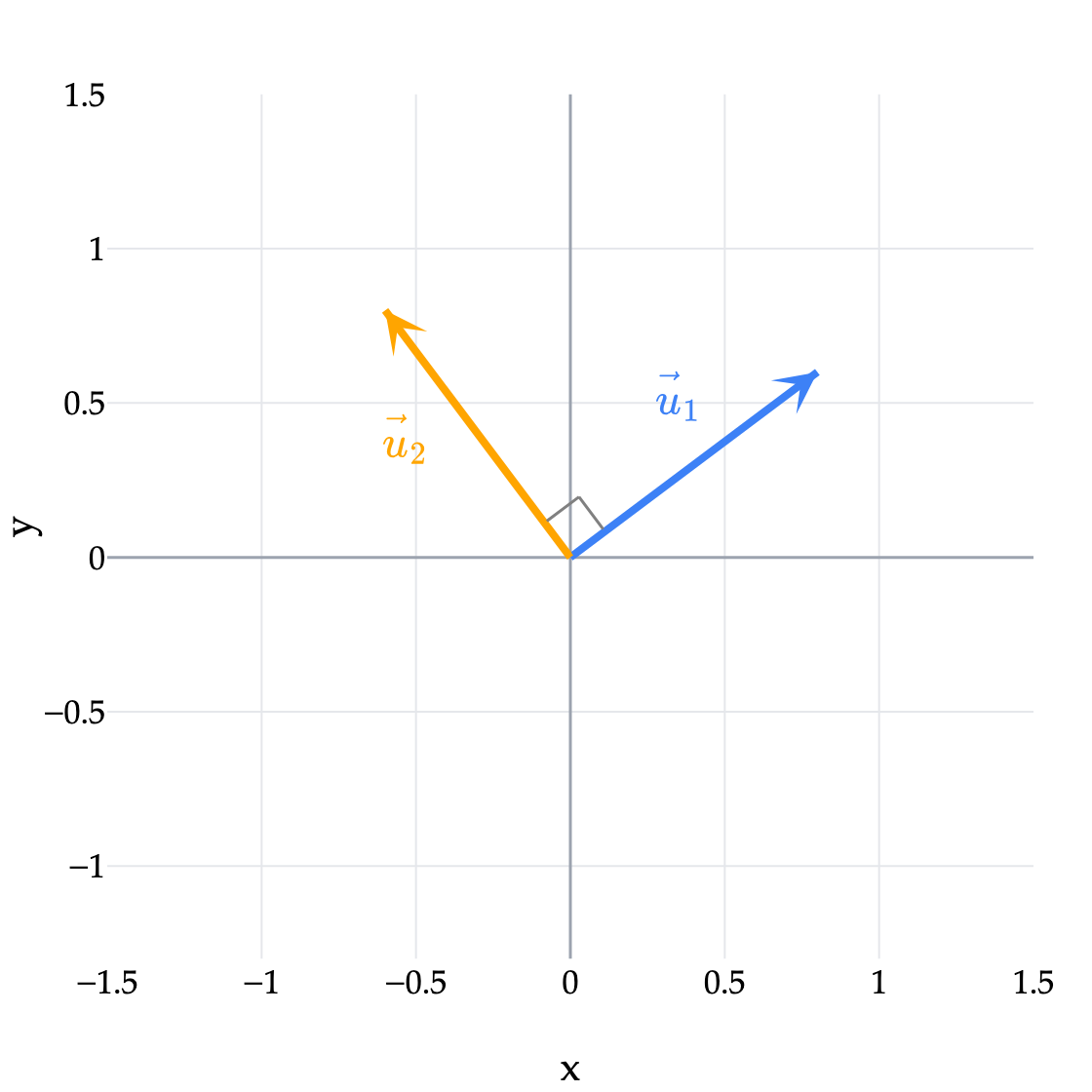
By Chapter 1.6, they are orthogonal. This pair is an orthonormal basis of R2\mathbb R^2.

Image produced in Jupyter

The pair (u⃗1,u⃗2)(\vec u_1,\vec u_2) is an orthonormal basis of R2\mathbb{R}^2.

We can choose a different pair of perpendicular unit directions. Let

w⃗1=[−1212],w⃗2=[−12−12].\vec w_1= \begin{bmatrix} -\frac{1}{\sqrt{2}}\\[2pt] \frac{1}{\sqrt{2}} \end{bmatrix}, \qquad \vec w_2= \begin{bmatrix} -\frac{1}{\sqrt{2}}\\[2pt] -\frac{1}{\sqrt{2}} \end{bmatrix}.

Each vector has squared length 1/2+1/2=11/2+1/2=1, and

w⃗1⋅w⃗2=12−12=0.\vec w_1\cdot\vec w_2=\frac12-\frac12=0.

So (w⃗1,w⃗2)(\vec w_1,\vec w_2) is also an orthonormal basis. There are many choices of orthonormal basis, just as there are many choices of direction vector for a line.
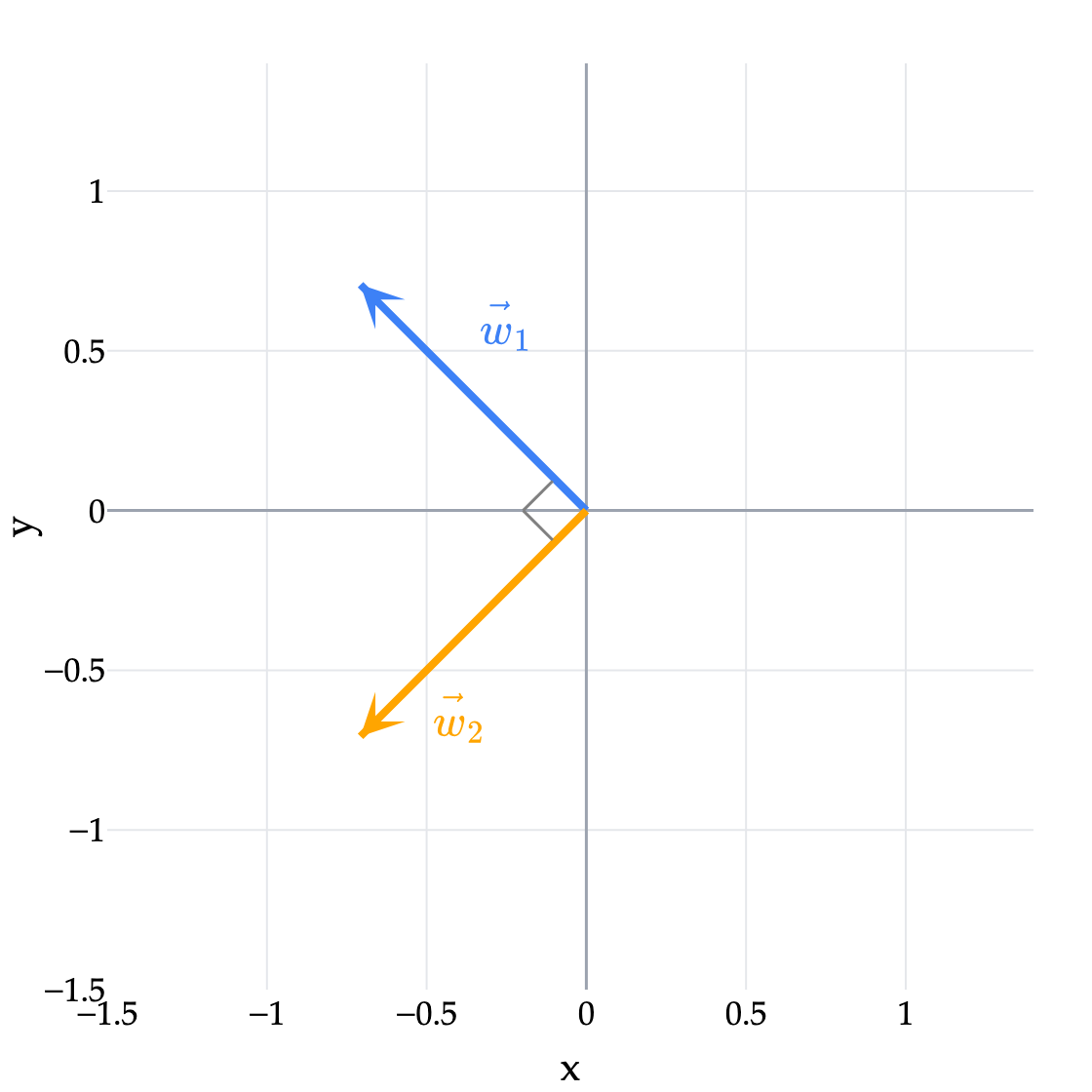
Image produced in Jupyter

An orthonormal basis is not unique.


Finding coefficients using dot products

An orthonormal basis gives us two perpendicular directions. Every vector can be written uniquely as a sum of multiples of those directions. How can we find the two coefficients?

Let u⃗1,u⃗2\vec u_1,\vec u_2 be an orthonormal basis of R2\mathbb{R}^2.

Let v⃗\vec v be any vector in R2\mathbb{R}^2.

Then

v⃗=au⃗1+bu⃗2\vec v=a\vec u_1+b\vec u_2

for some scalars a,ba,b. The figure below shows this decomposition by completing a rectangle.
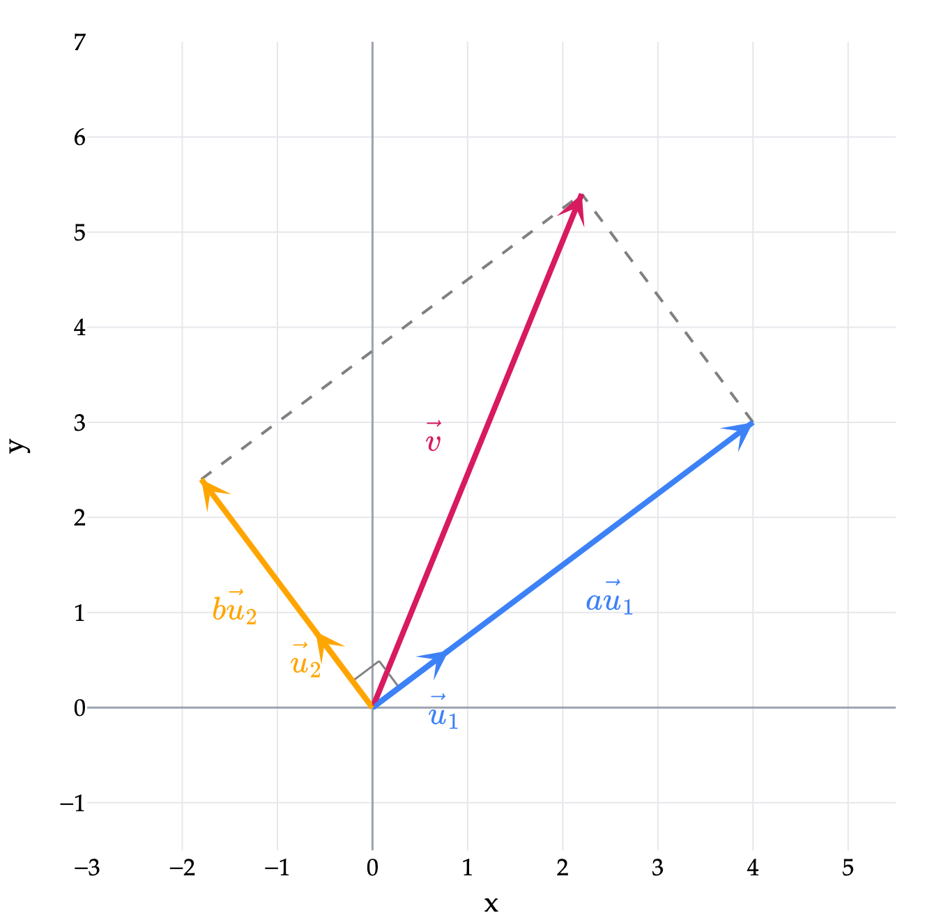
Image produced in Jupyter

v⃗=au⃗1+bu⃗2\vec v=a\vec u_1+b\vec u_2 with respect to the orthonormal directions u⃗1\vec u_1 and u⃗2\vec u_2.

The decomposition v⃗=au⃗1+bu⃗2\vec v=a\vec u_1+b\vec u_2 with respect to the orthonormal directions u⃗1\vec u_1 and u⃗2\vec u_2.

But how do we find a,ba,b?

The distributive and scalar-multiplication properties from Chapter 1.6 let us isolate one coefficient at a time. Take the dot product with u⃗1\vec u_1:

v⃗⋅u⃗1=(au⃗1+bu⃗2)⋅u⃗1=a(u⃗1⋅u⃗1)+b(u⃗2⋅u⃗1).\vec v\cdot \vec u_1 = (a\vec u_1+b\vec u_2)\cdot \vec u_1 = a(\vec u_1\cdot \vec u_1) + b(\vec u_2\cdot \vec u_1).

Since u⃗1\vec u_1 is a unit vector,

u⃗1⋅u⃗1=1.\vec u_1\cdot \vec u_1=1.

Since u⃗1\vec u_1 and u⃗2\vec u_2 are orthogonal,

u⃗2⋅u⃗1=0.\vec u_2\cdot \vec u_1=0.

Therefore

v⃗⋅u⃗1=a.\vec v\cdot \vec u_1=a.

Similarly,

b=v⃗⋅u⃗2.b=\vec v\cdot \vec u_2.

So

v⃗=(v⃗⋅u⃗1)u⃗1+(v⃗⋅u⃗2)u⃗2.\vec v = (\vec v\cdot \vec u_1)\vec u_1 + (\vec v\cdot \vec u_2)\vec u_2.

Representing the same vector in different bases

Let

v⃗=[75].\vec v= \begin{bmatrix} 7\\ 5 \end{bmatrix}.

Using the standard basis

For the standard basis

(e⃗1,e⃗2)=([10],[01]),(\vec e_1,\vec e_2) = \left( \begin{bmatrix} 1\\ 0 \end{bmatrix}, \begin{bmatrix} 0\\ 1 \end{bmatrix} \right),

we have

v⃗⋅e⃗1=[75]⋅[10]=7,\vec v\cdot \vec e_1 = \begin{bmatrix} 7\\ 5 \end{bmatrix} \cdot \begin{bmatrix} 1\\ 0 \end{bmatrix} = 7,

and

v⃗⋅e⃗2=[75]⋅[01]=5.\vec v\cdot \vec e_2 = \begin{bmatrix} 7\\ 5 \end{bmatrix} \cdot \begin{bmatrix} 0\\ 1 \end{bmatrix} = 5.

Therefore

(v⃗⋅e⃗1)e⃗1+(v⃗⋅e⃗2)e⃗2=7e⃗1+5e⃗2=[70]+[05]=[75].(\vec v\cdot \vec e_1)\vec e_1 + (\vec v\cdot \vec e_2)\vec e_2 = 7\vec e_1+5\vec e_2 = \begin{bmatrix} 7\\ 0 \end{bmatrix} + \begin{bmatrix} 0\\ 5 \end{bmatrix} = \begin{bmatrix} 7\\ 5 \end{bmatrix}.

Using a different orthonormal basis

Now take the orthonormal basis

(u⃗1,u⃗2)=([4535],[−3545]).(\vec u_1,\vec u_2) = \left( \begin{bmatrix} \frac45\\[2pt] \frac35 \end{bmatrix}, \begin{bmatrix} -\frac35\\[2pt] \frac45 \end{bmatrix} \right).

Then

v⃗⋅u⃗1=[75]⋅[4535]=285+155=435.\vec v\cdot \vec u_1 = \begin{bmatrix} 7\\ 5 \end{bmatrix} \cdot \begin{bmatrix} \frac45\\[2pt] \frac35 \end{bmatrix} = \frac{28}{5}+\frac{15}{5} = \frac{43}{5}.

Also,

v⃗⋅u⃗2=[75]⋅[−3545]=−215+205=−15.\vec v\cdot \vec u_2 = \begin{bmatrix} 7\\ 5 \end{bmatrix} \cdot \begin{bmatrix} -\frac35\\[2pt] \frac45 \end{bmatrix} = -\frac{21}{5}+\frac{20}{5} = -\frac15.

So

v⃗=435u⃗1−15u⃗2.\vec v = \frac{43}{5}\vec u_1 - \frac15 \vec u_2.

The coefficient −1/5-1/5 means the second component points opposite to u⃗2\vec u_2. The vector itself is still [75]\begin{bmatrix}7\\5\end{bmatrix}.