In Chapter 1.4, we drew the vector
along with and . When drawn from the origin, all three arrows lie on the same line.
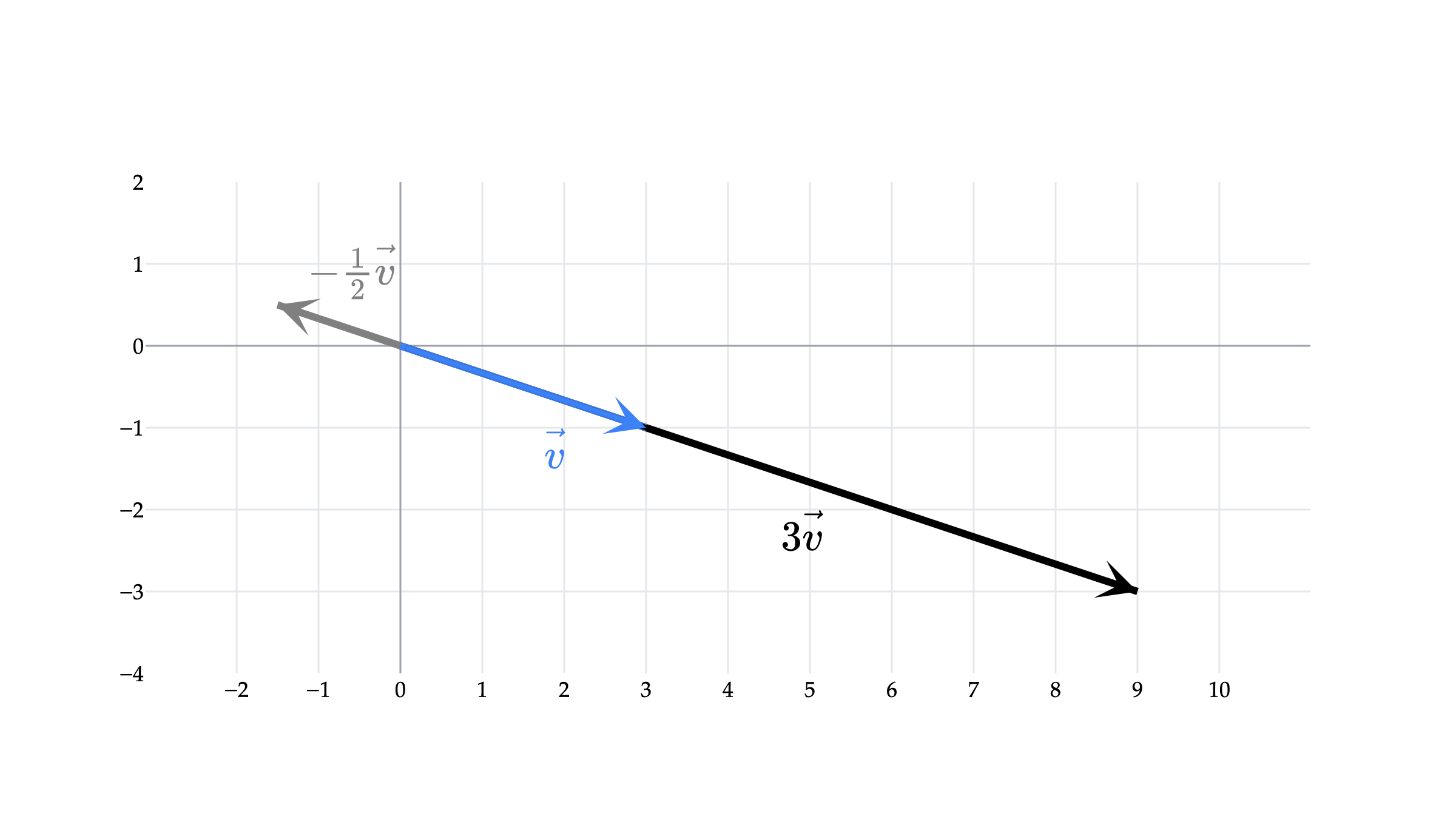
and its scalar multiples lie on the same line.
What if we drew every scalar multiple of ? Positive multiples extend along one direction, negative multiples extend along the opposite direction, and gives the origin. Together, they fill the entire line!
We’ll call this collection the span of and connect it to a familiar line equation. Then we’ll use orthogonality from Chapter 1.6 to describe the same line using a perpendicular vector.
Homogeneous and nonhomogeneous equations
A line in has an equation , where and are not both zero. Let’s start with
This line passes through the origin: substituting gives .
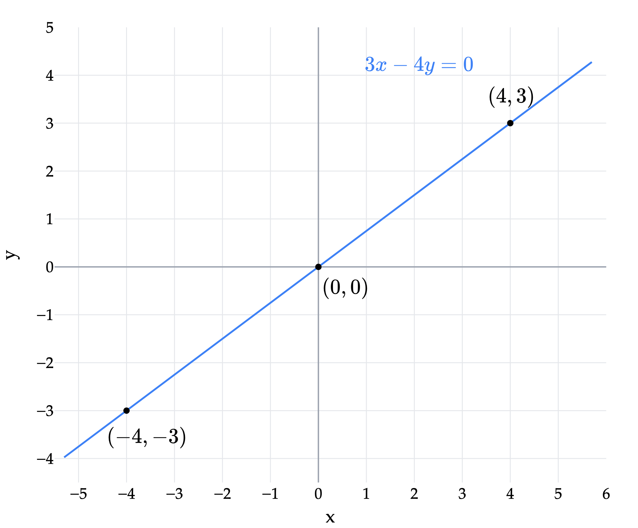
The line passes through the origin.
What happens if we change the right-hand side from 0 to 7? The origin no longer satisfies the equation, since . Instead, describes a parallel line.
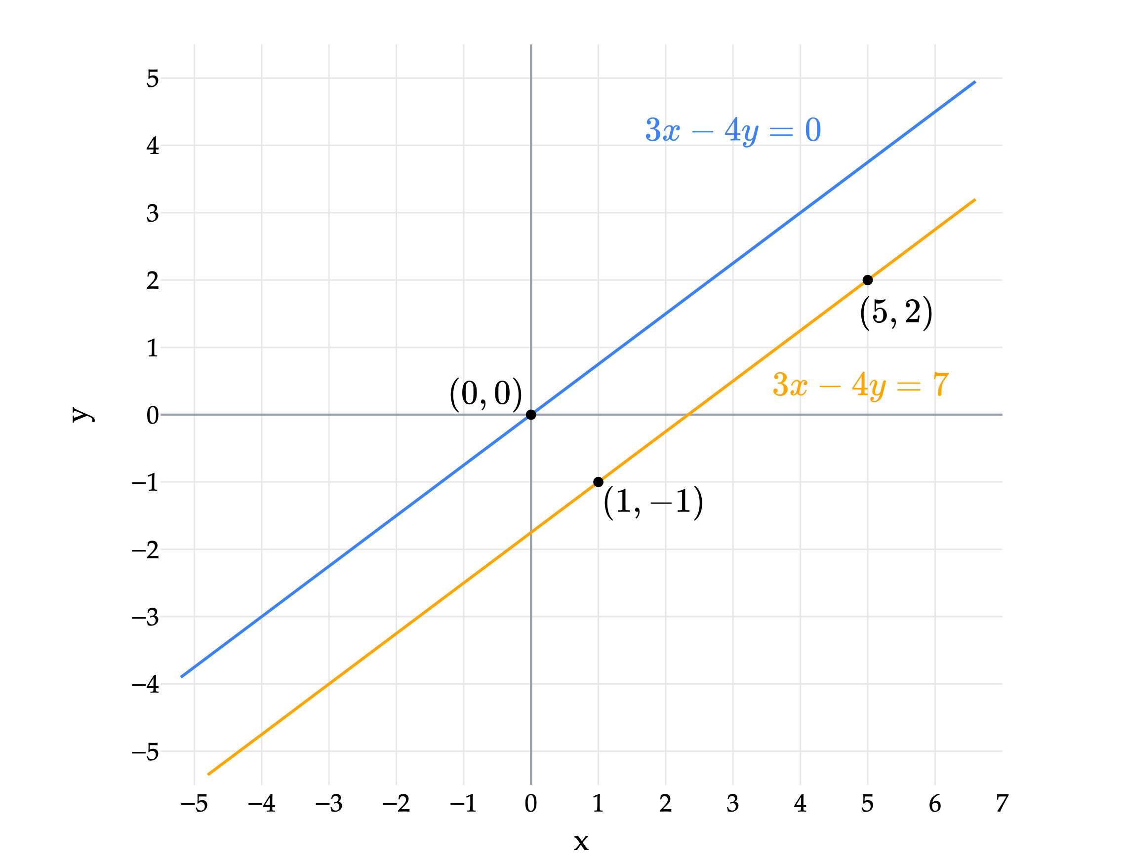
The lines and are parallel.
Keeping and fixed while varying gives parallel lines. For example, describes every line parallel to .
We’ll first focus on the homogeneous case: lines through the origin.
Lines as spans
The opening example suggests a second way to describe a line through the origin: take all scalar multiples of one nonzero vector along it.
For , let’s use
Every point on has the form for some scalar . Equivalently, we can write
This is a parametric form of the line. The scalar is called the parameter: each value of gives a point on the line, and letting range over all real numbers gives the entire line.
Drag the slider below to change and watch sweep along the line. Positive and negative values give opposite directions; when , the vector is the zero vector.
Drag the slider: the endpoint of stays on . The slider shows part of the line; can be any real number.
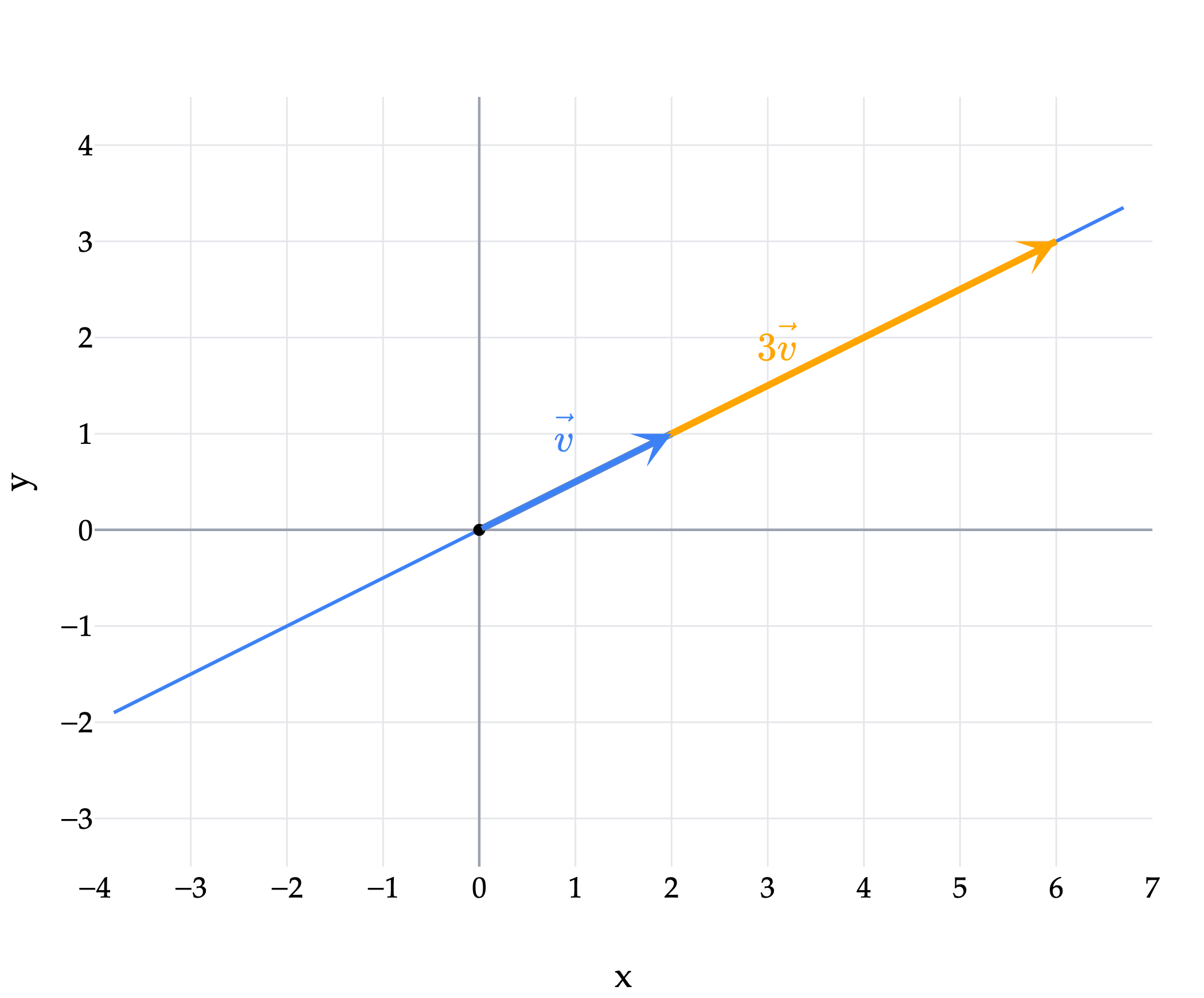
So . We could have picked any nonzero vector along this line, such as
Multiplying by a nonzero scalar changes the length, and possibly reverses the direction, as we saw in Chapter 1.5. It does not change the line that the vector spans:
Normal vectors and line equations
In Chapter 1.6, we learned that two vectors are orthogonal exactly when their dot product is zero. We can use this fact to connect a line’s equation to its geometry.
Let’s return to . We’ll use to refer to the line through the origin perpendicular to .
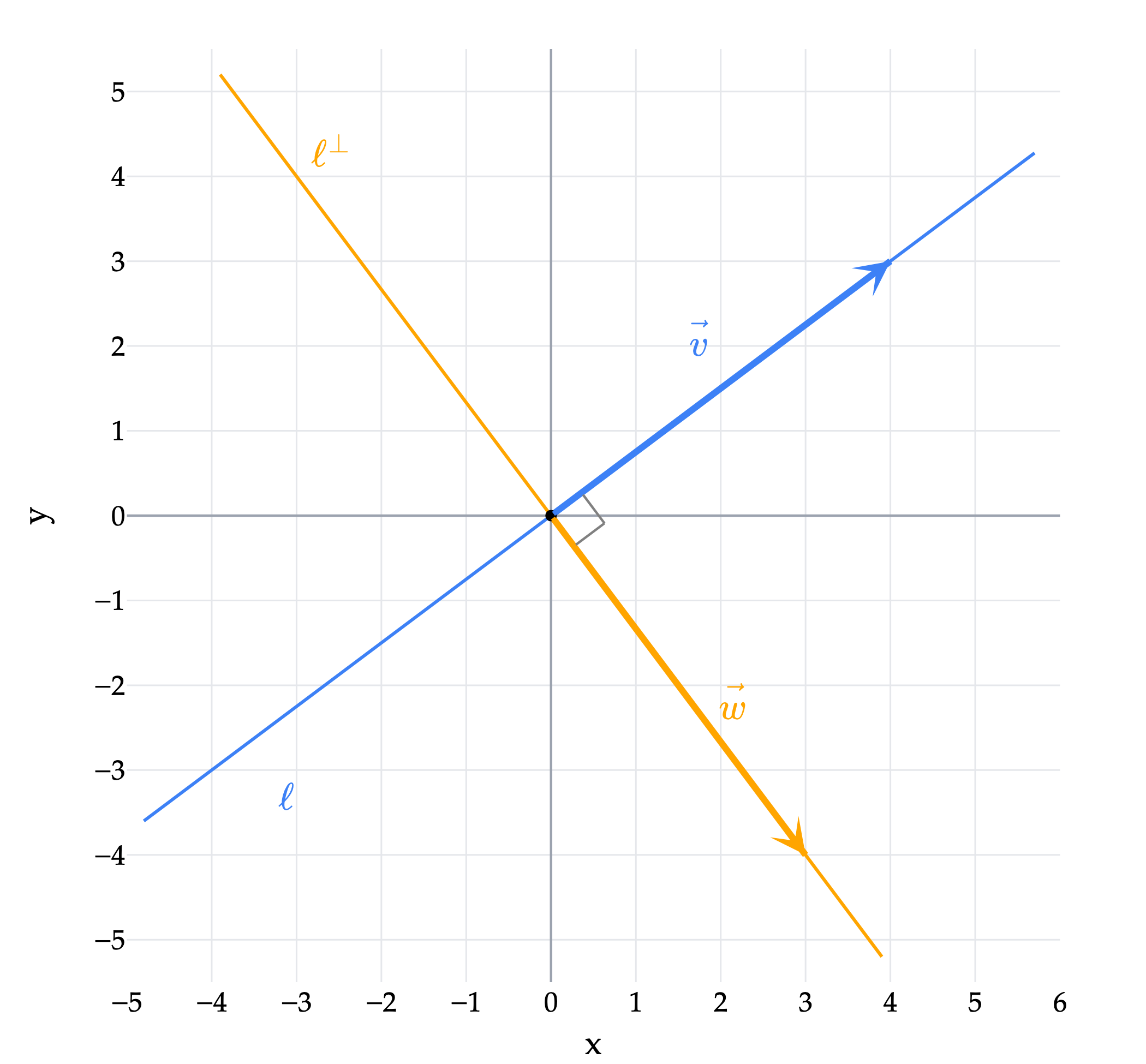
The normal vector is perpendicular to .
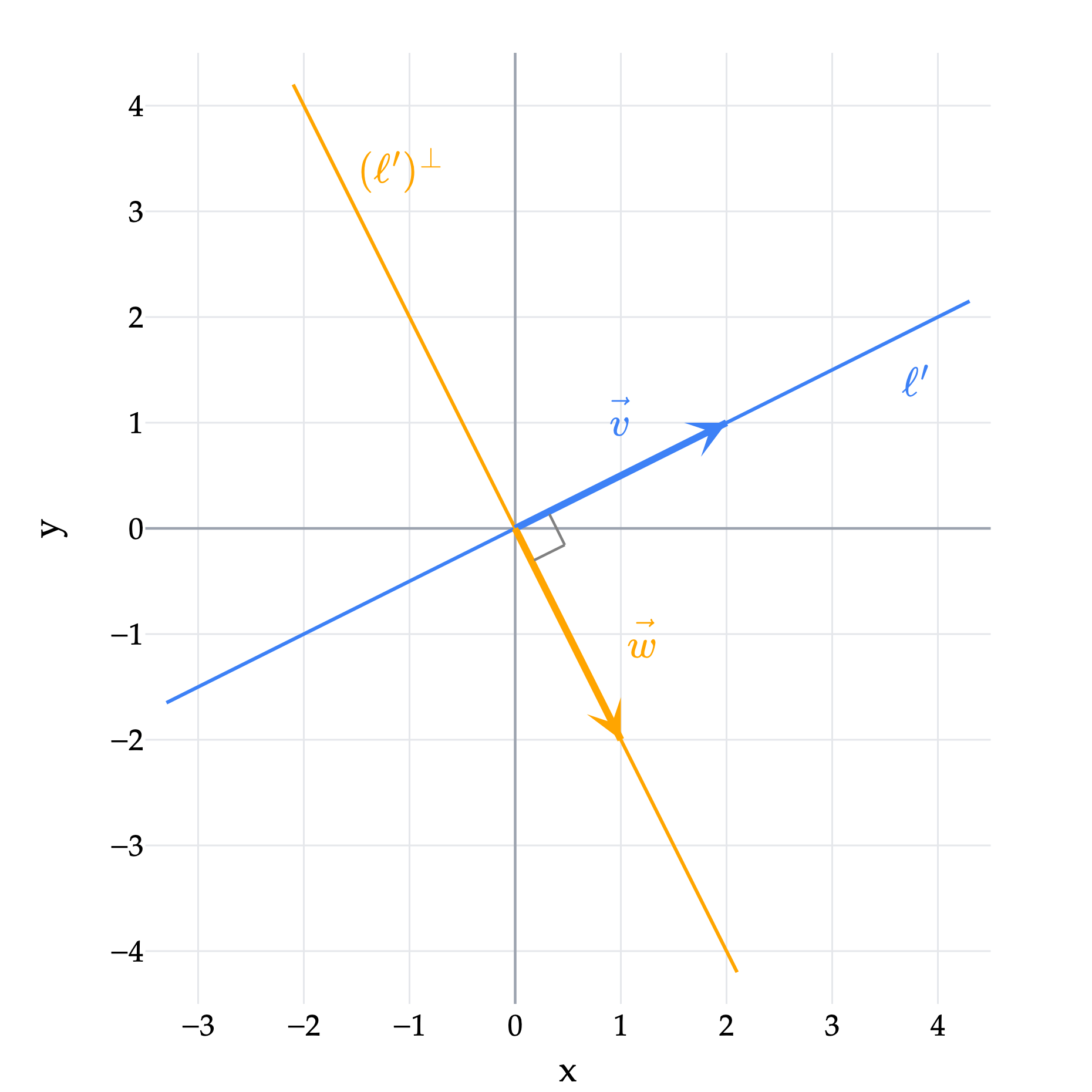
The coefficients of give us the vector
Why does this vector lie on ? We can rewrite the equation of as a dot product:
So lies on exactly when is orthogonal to .
We now have two ways to describe : take multiples of a vector along it, or use a vector perpendicular to it. With and ,
The roles reverse for : lies along it, and is perpendicular to it. Therefore,
Taking the dot product with gives the equation for .
A normal vector is not unique. For example, is also normal to , giving . This is just the original equation multiplied by 3, so it describes the same line.
Affine lines
Now let’s return to , which does not pass through the origin.
In Chapter 1.4, we saw that a vector represents a displacement and can be drawn from any starting point. We can use that idea to shift an entire line.
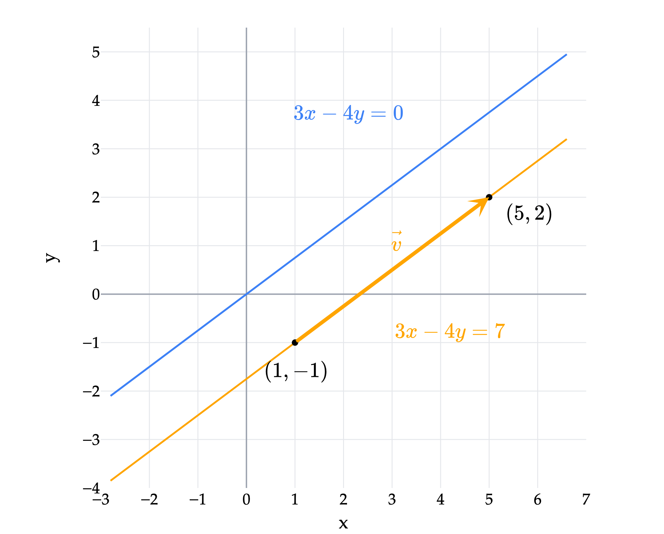
Starting at and adding takes us to .
The point lies on . Starting there and adding any multiple of takes us to another point on the line. The vector gives its direction, just as it did for .
So we can describe the line as
This gives the parametric form
Our starting point is not unique. For example, also lies on the line, so the same line is
Finding the constant from a point
Suppose we know a point on an affine line and a normal vector, but not its equation. How can we find the constant on the right-hand side?
Let be the position vector of the known point, let be a nonzero normal vector, and write
A point with position vector lies on the line exactly when the displacement is perpendicular to . Therefore,
In general, an affine line in through with nonzero normal vector has equation
The right-hand side is a constant: take the dot product of the normal vector with the known point’s position vector. For our line, and give , recovering .
For another example, consider the affine line in
To write an equation for this line, choose a nonzero vector perpendicular to its direction:
Then use the known point to find the constant:
The dot-product equation and its expanded form are
To check the result, substitute the parametric coordinates of the line:
This holds for every , as it should.
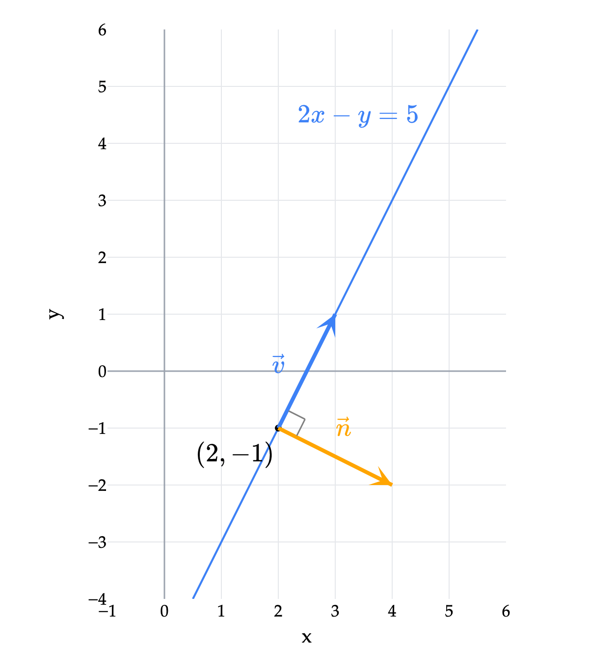
The line passes through . Its direction vector and normal vector are perpendicular.
Here’s a video reviewing how to find the equation of a line in .