2.2: Linear combinations - Math 124 Notes

Decomposing vectors¶

Using the concepts of vector addition and scalar multiplication, we can decompose vectors into sums of ‘standard vectors’. Let’s start again with an example to illustrate what we mean by this. Observe that

\begin{pmatrix}2 \\ 3\end{pmatrix} = \begin{pmatrix}2 \\ 0\end{pmatrix} + \begin{pmatrix}0 \\ 3\end{pmatrix} = 2\begin{pmatrix}1 \\ 0\end{pmatrix} + 3\begin{pmatrix}0 \\ 1\end{pmatrix} = 2\vec e_1 + 3\vec e_2,

(1)

where $\vec e_i$ denotes the vector whose $i$ -th entry is 1 and the other entries are all zero. These $\vec e_i$ are called the standard basis vectors. The process above shows how to decompose the vector $\begin{pmatrix}2\\3 \end{pmatrix}$ into sums of scalar multiples of the standard basis vectors.

Let’s look at some other examples and then generalize.

\begin{pmatrix}-3 \\ -1\end{pmatrix} = \begin{pmatrix}-3 \\ 0\end{pmatrix} + \begin{pmatrix}0 \\ -1\end{pmatrix} = (-3)\begin{pmatrix}1 \\ 0\end{pmatrix} + (-1)\begin{pmatrix}0 \\ 1\end{pmatrix} = -3\vec e_1 - \vec e_2,

(2)

\begin{pmatrix} 1\\3\\-4\end{pmatrix} = \begin{pmatrix} 1\\0\\0\end{pmatrix} + \begin{pmatrix} 0\\3\\0\end{pmatrix} + \begin{pmatrix} 0\\0\\-4\end{pmatrix} = \begin{pmatrix} 1\\0\\0\end{pmatrix} + 3\begin{pmatrix} 0\\1\\0\end{pmatrix} + (-4)\begin{pmatrix} 0\\0\\1\end{pmatrix} = \vec e_1 + 3\vec e_2 - 4\vec e_3.

(3)

In general, this decomposition can be expressed as

\begin{pmatrix} x_1 \\ \vdots \\ x_n \end{pmatrix} = x_1 \vec e_1 + \cdots + x_n \vec e_n.

(4)

We see that any vector in $\mathbb{R}^n$ , i.e. any vector with $n$ entries, can be decomposed into a sum of scalar multiples of $\vec e_1, \ldots, \vec e_n$ .

What does this decomposition mean geometrically, given our interpretation of the sum of two vectors as forming triangles? Let’s focus on the case of two dimensions and look at following illustration that describe the examples above:

from IPython.display import display, HTML
import plotly.io as pio
import numpy as np

# Set default renderer to high-DPI static image
pio.renderers.default = "png"
display(HTML(
    '<script type="text/javascript" async src="https://cdnjs.cloudflare.com/ajax/libs/mathjax/2.7.1/MathJax.js?config=TeX-MML-AM_SVG"></script>'
))

# ---
from utils import plot_vectors_non_origin

# Define vectors: (((start_x, start_y), (end_x, end_y)), color, label)
vectors = [
    # 1. Scaled basis vectors along the x-axis
    (((0, 0), (2, 0)), 'blue', r'$2\vec{e}_1$'),
    (((0, 0), (-3, 0)), 'red', r'$-3\vec{e}_1$'),
    
    # 2. The standard unit vectors (gold, drawn so they sit on top)
    (((0, 0), (1, 0)), 'rgba(244, 180, 0, 0.9)', r'$\vec{e}_1$'),
    (((0, 0), (0, 1)), '#f4b400', r'$\vec{e}_2$'),
    
    # 3. Vertical components (head-to-tail)
    (((2, 0), (2, 3)), 'blue', r'$3\vec{e}_2$'),
    (((-3, 0), (-3, -1)), 'red', r'$-\vec{e}_2$'),
    
    # 4. The resultant decomposed vectors (formatted as column vectors)
    # Note the \\\\ required for matrix line breaks in Plotly
    (((0, 0), (2, 3)), 'green', r'$\begin{pmatrix} 2 \\ 3 \end{pmatrix}$'),
    (((0, 0), (-3, -1)), 'teal', r'$\begin{pmatrix} -3 \\ -1 \end{pmatrix}$')
]

# Adjust label offsets 
fig = plot_vectors_non_origin(vectors, vdeltax=0.35, vdeltay=0.35)

# Lock the aspect ratio so the grid is perfectly square
fig.update_layout(width=700, height=600, yaxis_scaleanchor="x")

# Set the grid range to frame both decompositions clearly in opposing quadrants
fig.update_xaxes(range=[-4, 4], tickvals=np.arange(-4, 5))
fig.update_yaxes(range=[-3, 5], tickvals=np.arange(-3, 6))

fig.show(scale=3)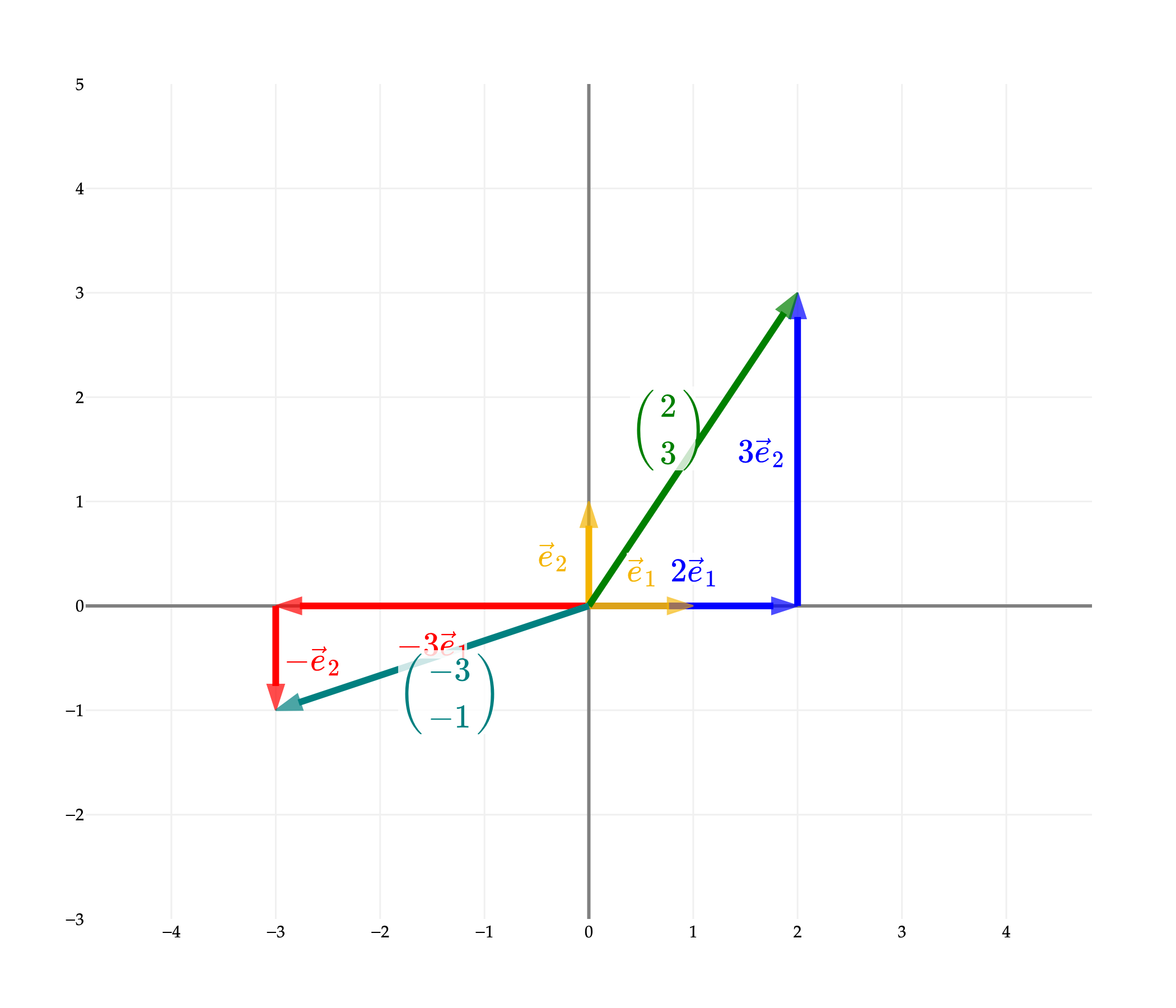

Loading...

Recall that any vector in $\mathbb{R}^2$ can be decomposed as a sum of scalar multiples of $\vec e_1$ and $\vec e_2$ . Geometrically, this means that any vector in $\mathbb{R}^2$ can be decomposed as a sum of two vectors parallel to the $x$ -axis and the $y$ -axis.

The same principal holds for vectors of dimension 3: any vector in $\mathbb{R}^3$ can be decomposed as a sum of three vectors, each parallel to the $x$ , $y$ , and $z$ -axes. The following depicts the decomposition of vector $\begin{pmatrix} 2\\3\\5\end{pmatrix}$ into $2\vec e_1 + 3\vec e_2 + 5\vec e_3$ .

from IPython.display import display, HTML
import plotly.io as pio
import numpy as np

# Set default renderer to high-DPI static image
pio.renderers.default = "png"
display(HTML(
    '<script type="text/javascript" async src="https://cdnjs.cloudflare.com/ajax/libs/mathjax/2.7.1/MathJax.js?config=TeX-MML-AM_SVG"></script>'
))

# ---
from utils import plot_vectors_non_origin

# Define 3D vectors: (((start_x, start_y, start_z), (end_x, end_y, end_z)), color, label)
vectors = [
    # 1. The scaled component along the x-axis (drawn first so it sits underneath e_1)
    (((0, 0, 0), (2, 0, 0)), 'red', '2<i>e</i><sub>1</sub>\u20D7'),
    
    # 2. The standard unit basis vectors (gold, drawn at the origin)
    (((0, 0, 0), (1, 0, 0)), 'rgba(244, 180, 0, 0.9)', '<i>e</i><sub>1</sub>\u20D7'),
    (((0, 0, 0), (0, 1, 0)), '#f4b400', '<i>e</i><sub>2</sub>\u20D7'),
    (((0, 0, 0), (0, 0, 1)), '#f4b400', '<i>e</i><sub>3</sub>\u20D7'),
    
    # 3. The remaining scaled components, connected head-to-tail
    (((2, 0, 0), (2, 3, 0)), 'blue', '3<i>e</i><sub>2</sub>\u20D7'),
    (((2, 3, 0), (2, 3, 5)), 'purple', '5<i>e</i><sub>3</sub>\u20D7'),
    
    # 4. The resultant decomposed vector from the origin
    (((0, 0, 0), (2, 3, 5)), 'green', '')
]

# Adjust offsets for the 3D labels to prevent overlap with the lines
fig = plot_vectors_non_origin(vectors, vdeltax=0.3, vdeltay=0.3, vdeltaz=0.3)

# Frame the grid, forcing integer ticks (dtick=1) to keep the axes clean
fig.update_layout(
    width=700, 
    height=600,
    scene=dict(
        xaxis=dict(range=[-1, 3], dtick=1),
        yaxis=dict(range=[-1, 4], dtick=1),
        zaxis=dict(range=[-1, 6], dtick=1),
        aspectratio=dict(x=1, y=1, z=1.2) # Slightly elongated z-axis to match the coordinates
    )
)

fig.show(scale=5)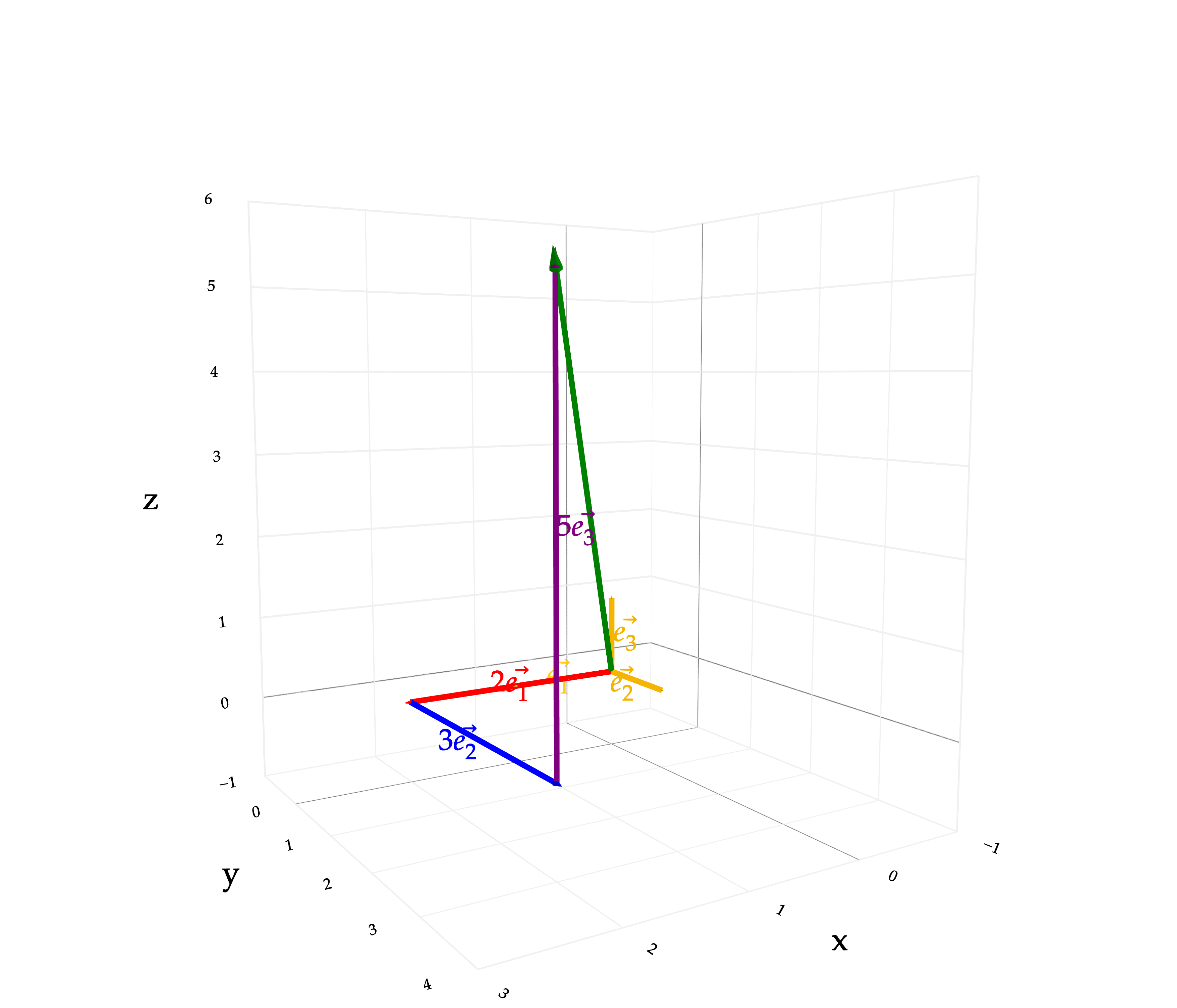

Loading...

Linear combinations¶

We have seen that any vector in $\mathbb{R}^2$ can be expressed as a sum of scalar multiples of $\vec e_1$ and $\vec e_2$ . This is a bit mouthful, and we will instead say that any vector in $\mathbb{R}^2$ is the ‘linear combination’ of $\vec e_1$ and $\vec e_2$ .

The formal definition of a linear combination does not need to involve the standard basis vectors $\vec e_i$ . A linear combination of two vectors $\vec u$ and $\vec v$ is any sum of their scalar multiples, i.e. any vector of the form

a \vec u + b \vec v

(5)

for scalars $a$ and $b$ . More generally, we define a linear combination of $n$ vectors $\vec v_1, \ldots \vec v_n$ to be any vector of the form

a_1 \vec v_1 + \cdots + a_n \vec v_n

(6)

for scalars $a_1, \ldots, a_n$ . Again, note that all vectors in $\mathbb{R}^n$ are linear combinations of $\vec e_1, \ldots, \vec e_n$ .

This definition also applies to the case where we only have one vector $\vec v_1$ ; a linear combination of $\vec v_1$ is any scalar multiple of $\vec v_1$ .

Lines and planes as spans¶

A concept closely related to linear combinations is span. The span of vectors $\vec v_1,\ldots,\vec v_n$ is simply the set of all linear combinations of $\vec v_1,\ldots,\vec v_n$ . We denote the span by

\langle \vec v_1 ,\ldots, \vec v_n\rangle.

(7)

Note that in set-builder notation, the span can be written as

\langle \vec v_1 ,\ldots, \vec v_n\rangle = \left\{ a_1 \vec v_1 + \cdots + a_n \vec v_n: a_1, \ldots, a_n \in \mathbb{R}\right\}.

(8)

For instance, we have seen that $\mathbb{R}^n$ is the span of the standard basis vectors $\vec e_1, \ldots \vec e_n$ , hence allowing us to write $\mathbb{R}^n = \langle \vec e_1, \ldots, \vec e_n\rangle$ .

For now we will focus on spans of vectors in $\mathbb{R}^2$ and $\mathbb{R}^3$ . If $\mathbb{R}^3$ is the span of the standard basis vectors $\vec e_1, \vec e_2, \vec e_3$ , what is the span of just $\vec e_1, \vec e_2$ ? We obtain vectors of the following form:

a\vec e_1 + b\vec e_2 = a \begin{bmatrix} 1\\0\\0 \end{bmatrix} + b \begin{bmatrix} 0\\1\\0 \end{bmatrix} = \begin{bmatrix} a\\b\\0 \end{bmatrix}

(9)

for all scalars $a,b$ . In other words, we obtain all vectors with the third entry being zero.

Geometrically, the span corresponds to the $x$ - $y$ plane inside the three-dimensional Euclidean space depicted in blue:

from IPython.display import display, HTML
import plotly.io as pio
import plotly.graph_objects as go
import numpy as np

# Set default renderer to high-DPI static image
pio.renderers.default = "png"
display(HTML(
    '<script type="text/javascript" async src="https://cdnjs.cloudflare.com/ajax/libs/mathjax/2.7.1/MathJax.js?config=TeX-MML-AM_SVG"></script>'
))

# ---
from utils import plot_vectors_non_origin

# 1. Define the standard basis vectors to orient the viewer
vectors = [
    (((0, 0, 0), (1.5, 0, 0)), 'red', '<i>e</i><sub>1</sub>\u20D7'),
    (((0, 0, 0), (0, 1.5, 0)), 'green', '<i>e</i><sub>2</sub>\u20D7'),
    (((0, 0, 0), (0, 0, 1.5)), 'blue', '<i>e</i><sub>3</sub>\u20D7')
]

# Create the base figure with the vectors
fig = plot_vectors_non_origin(vectors, vdeltax=0.4, vdeltay=0.4, vdeltaz=0.4)

# 2. Define the grid boundaries for the planes
# We only need the extreme corners (2 points per axis) to draw a flat square
x_vals = np.array([-4, 4])
y_vals = np.array([-4, 4])
z_vals = np.array([-4, 4])

# --- XY Plane (z=0) - Blue tint ---
x_xy, y_xy = np.meshgrid(x_vals, y_vals)
z_xy = np.zeros_like(x_xy)
fig.add_trace(go.Surface(
    x=x_xy, y=y_xy, z=z_xy, 
    colorscale=[[0, 'rgba(100, 150, 250, 0.3)'], [1, 'rgba(100, 150, 250, 0.3)']],
    showscale=False, hoverinfo='skip'
))

# --- XZ Plane (y=0) - Red tint ---
x_xz, z_xz = np.meshgrid(x_vals, z_vals)
y_xz = np.zeros_like(x_xz)
fig.add_trace(go.Surface(
    x=x_xz, y=y_xz, z=z_xz,
    colorscale=[[0, 'rgba(100, 250, 150, 0.3)'], [1, 'rgba(100, 250, 150, 0.3)']],
    
    showscale=False, hoverinfo='skip'
))

# --- YZ Plane (x=0) - Green tint ---
y_yz, z_yz = np.meshgrid(y_vals, z_vals)
x_yz = np.zeros_like(y_yz)
fig.add_trace(go.Surface(
    x=x_yz, y=y_yz, z=z_yz, 
    colorscale=[[0, 'rgba(250, 100, 150, 0.3)'], [1, 'rgba(250, 100, 150, 0.3)']],
    showscale=False, hoverinfo='skip'
))

# 3. Format the layout for a clean schematic look
# Using tickvals limits the labels to just the outer edges and origin
schematic_ticks = [-4, 0, 4]

fig.update_layout(
    width=700, 
    height=600,
    scene=dict(
        xaxis=dict(range=[-4, 4], tickvals=schematic_ticks),
        yaxis=dict(range=[-4, 4], tickvals=schematic_ticks),
        zaxis=dict(range=[-4, 4], tickvals=schematic_ticks),
        aspectratio=dict(x=1, y=1, z=1) # Perfectly cubic
    )
)

fig.show(scale=5)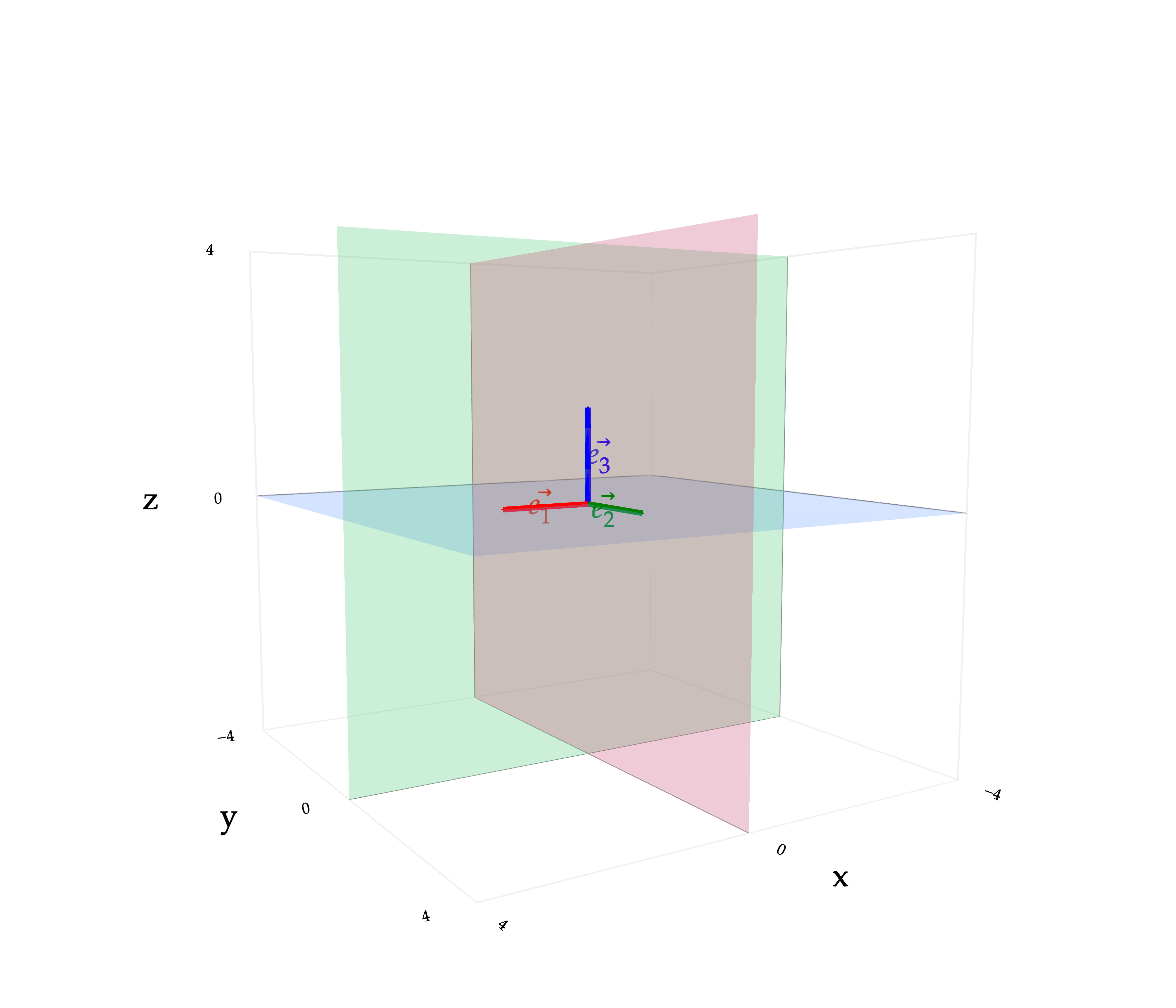

Loading...

We can similarly work out that

the span of $\vec e_2, \vec e_3$ form the $y$ - $z$ plane colored in red;
the span of $\vec e_1, \vec e_3$ form the $x$ - $z$ plane colored in green.

We can also think about spans of vectors other than the standard basis vectors. Let’s start with the simplest case where we only have one vector. What is the span of the vector $\vec v = \begin{bmatrix}1 \\ 2\end{bmatrix}$ ? It is the set of all multiples of $\vec v$ , which in the Euclidean plane corresponds to the following line through the origin:

from IPython.display import display, HTML
import plotly.io as pio
import plotly.graph_objects as go
import numpy as np

# Set default renderer to high-DPI static image
pio.renderers.default = "png"
display(HTML(
    '<script type="text/javascript" async src="https://cdnjs.cloudflare.com/ajax/libs/mathjax/2.7.1/MathJax.js?config=TeX-MML-AM_SVG"></script>'
))

# ---
from utils import plot_vectors

# 1. Define the vectors
vectors = [
    ((3, 6), 'rgba(100, 150, 250, 0.7)', r'$3\vec{v}$'),       
    ((-2, -4), 'rgba(0, 128, 0, 0.7)', r'$-2\vec{v}$'),        
    ((1, 2), '#f4b400', r'$\vec{v}$')                          
]

# Create the figure with the vectors
fig = plot_vectors(vectors, vdeltax=0.5, vdeltay=-0.2)

# 2. Add the continuous solid line representing the span
# We make it thick (width=8) but highly transparent (opacity=0.2)
fig.add_trace(go.Scatter(
    x=[-3.5, 4.5],
    y=[-7, 9],
    mode='lines',
    line=dict(color='rgba(128, 0, 128, 0.4)', width=5), 
    showlegend=False,
    hoverinfo='skip'
))

# 3. FIX THE CLUTTER (Z-Ordering)
# Plotly draws traces in the order they are added. The line was just added last (on top).
# This single line of Python tuple reassignment pushes the line to the absolute back.
fig.data = (fig.data[-1],) + fig.data[:-1]

# 4. Format the layout
fig.update_layout(width=600, height=700, yaxis_scaleanchor="x")
fig.update_xaxes(range=[-4, 5], tickvals=np.arange(-4, 6))
fig.update_yaxes(range=[-7, 8], tickvals=np.arange(-7, 9))

fig.show(scale=3)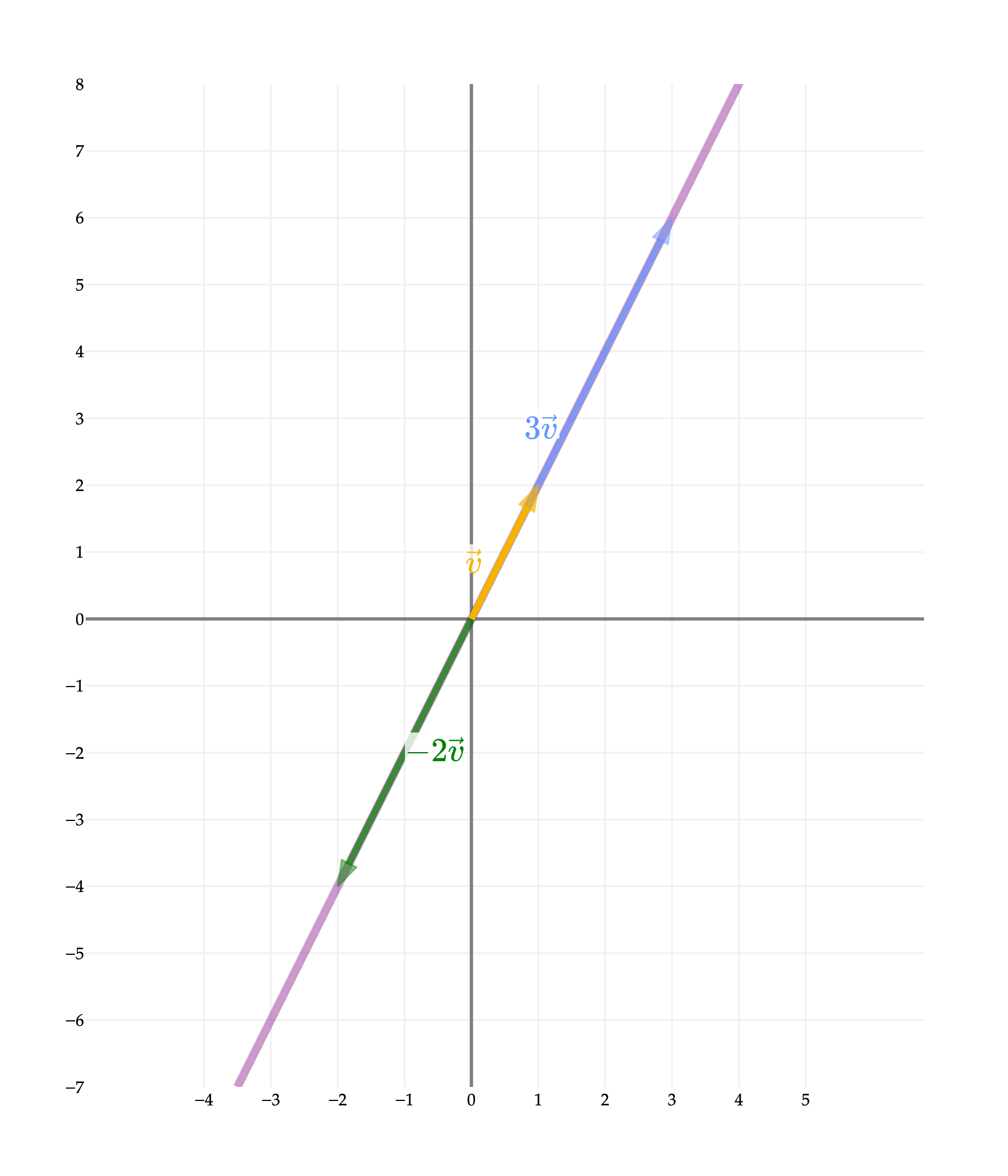

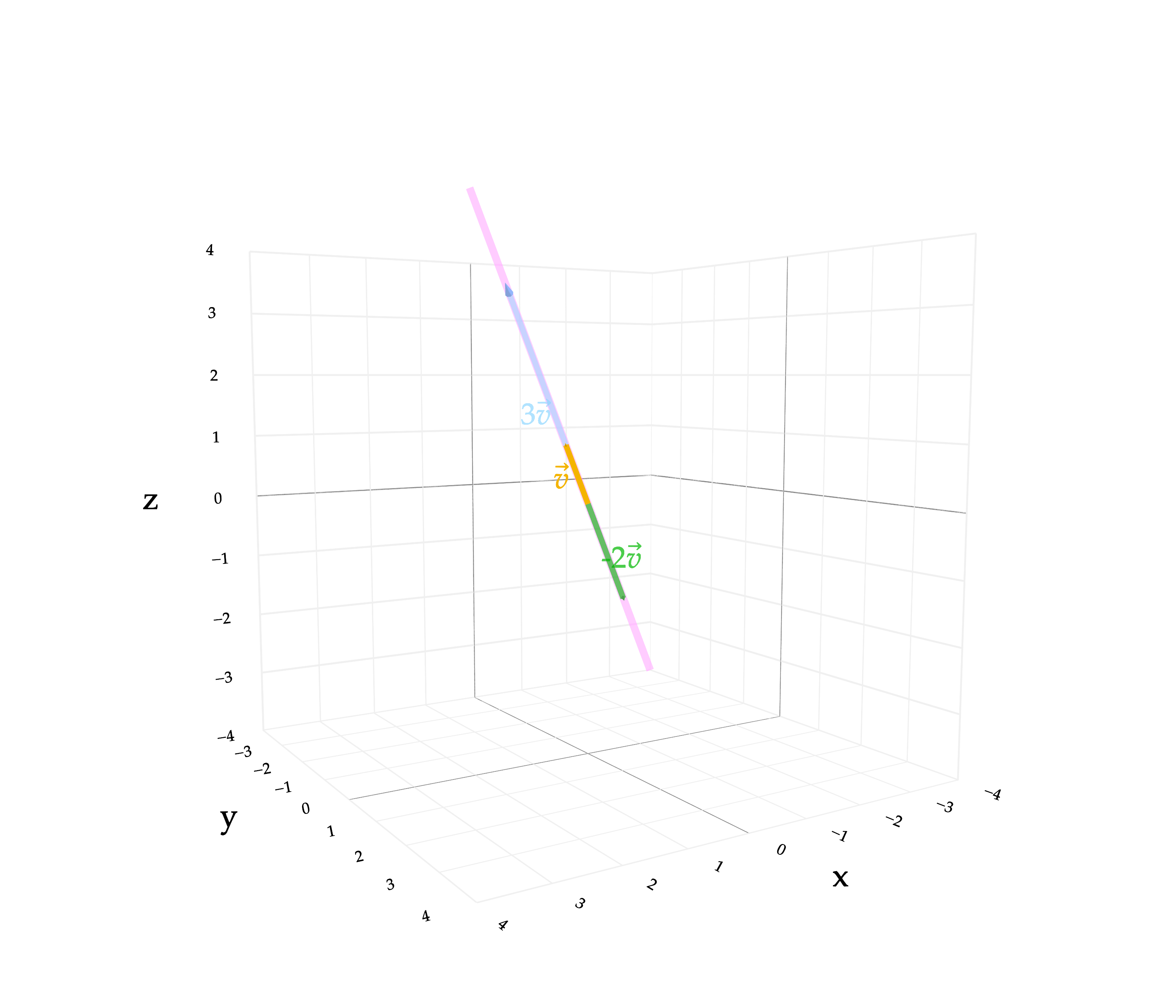
Loading...

Similarly, the span of a vector in $\mathbb{R}^3$ also traces out a line in three-dimensional Euclidean space. Here is an illustration for the vector $\vec v = \begin{bmatrix} 1\\1\\1\end{bmatrix}$ with some of its scalar multiples.

from IPython.display import display, HTML
import plotly.io as pio
import plotly.graph_objects as go
import numpy as np

# Set default renderer to high-DPI static image
pio.renderers.default = "png"
display(HTML(
    '<script type="text/javascript" async src="https://cdnjs.cloudflare.com/ajax/libs/mathjax/2.7.1/MathJax.js?config=TeX-MML-AM_SVG"></script>'
))

# ---
from utils import plot_vectors_non_origin

# 1. Define the 3D vectors
# Start/end coordinates: (((x0, y0, z0), (x1, y1, z1)), color, label)
vectors = [
    (((0, 0, 0), (3, 3, 3)), 'rgba(100, 150, 250, 0.7)', '3<i>v</i>\u20D7'),     # 3v (transparent blue)
    (((0, 0, 0), (-2, -2, -2)), 'rgba(0, 128, 0, 0.7)', '-2<i>v</i>\u20D7'),      # -2v (transparent green)
    (((0, 0, 0), (1, 1, 1)), '#f4b400', '<i>v</i>\u20D7')                         # The original vector v (solid gold)
]

# Create the figure
fig = plot_vectors_non_origin(vectors, vdeltax=0.5, vdeltay=0.5, vdeltaz=0.5)

# 2. Add the continuous solid line representing the span in 3D
# The line represents the parametric equation x=t, y=t, z=t
# Thick (width=8) but highly transparent (opacity=0.2) purple line
fig.add_trace(go.Scatter3d(
    x=[-4, 4],
    y=[-4, 4],
    z=[-4, 4],
    mode='lines',
    line=dict(color='rgba(128, 0, 128, 0.2)', width=8), 
    showlegend=False,
    hoverinfo='skip'
))

# 3. FIX THE CLUTTER (Z-Ordering)
# Push the line to the absolute back so it rests beneath the 3D arrows
fig.data = (fig.data[-1],) + fig.data[:-1]

# 4. Format the layout
# Frame the grid cleanly with integer ticks (dtick=1)
fig.update_layout(
    width=700, 
    height=600,
    scene=dict(
        xaxis=dict(range=[-4, 4], dtick=1),
        yaxis=dict(range=[-4, 4], dtick=1),
        zaxis=dict(range=[-4, 4], dtick=1),
        aspectratio=dict(x=1, y=1, z=1) # Keeps the 3D space perfectly cubic
    )
)

fig.show(scale=5)

Loading...