4.5: (P)LU factorization for all matrices

A factorization for every matrix¶

Multiplying by $P$ reorders the rows. When no row swaps are needed, we can take $P=I$ and write $A=LU$ .

The factor $L$ is always square. The new creature is $U$ : instead of necessarily being square, it always has the same shape as $A$ , $n\times d$ .

(n\times d)=(n\times n)(n\times d).

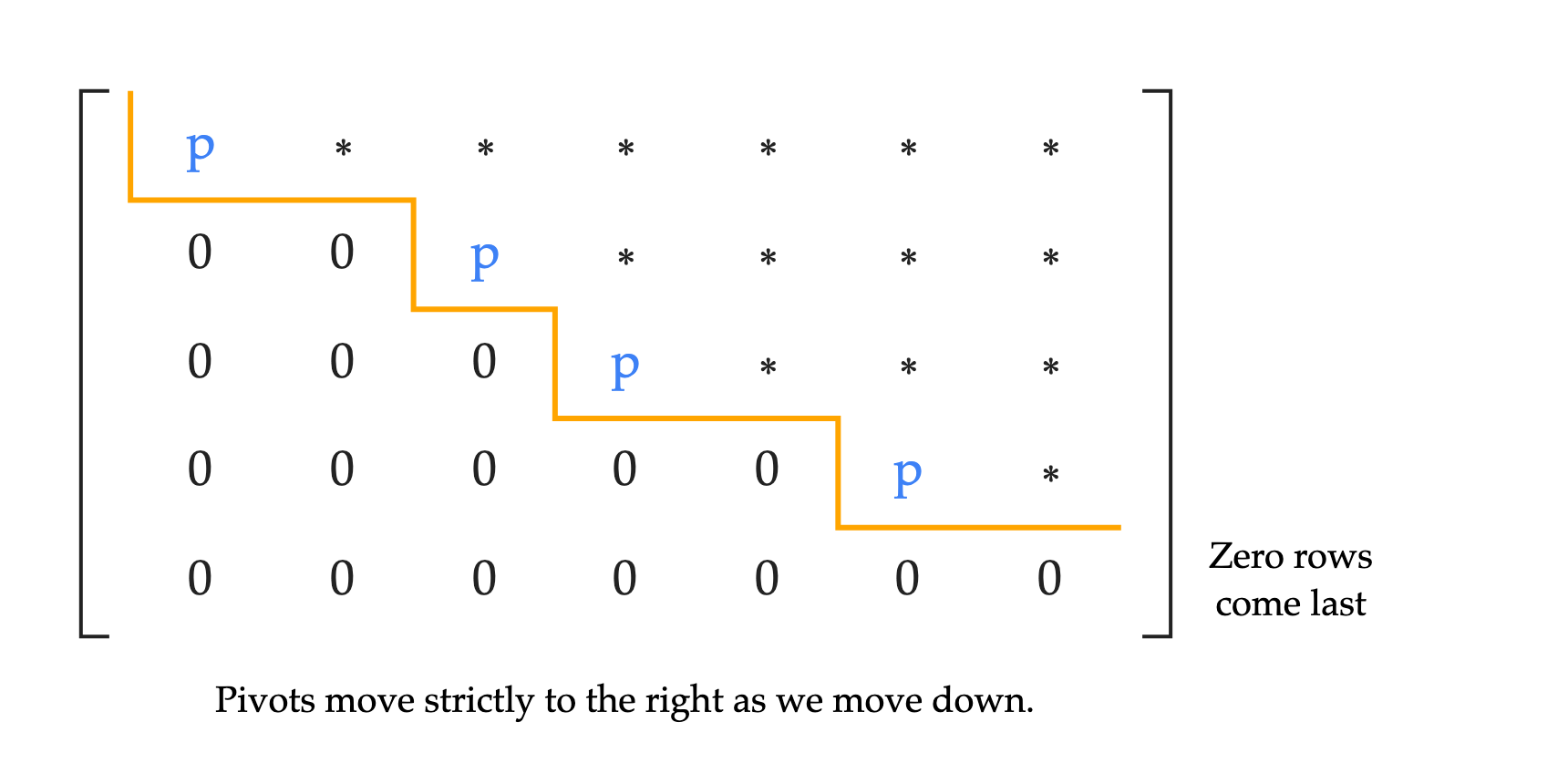
The role of $U$ is to give us a system that we can solve from the bottom up. For a general matrix, the useful pattern is a staircase: the first nonzero entries move to the right as we move down the rows, and any zero rows come last. This is row echelon form. It allows us to use the same approach for square and non-square matrices.

As before, we will find the factors by multiplying and matching entries. Chapter 4.6 gives an optional interpretation: $U$ is the result of using row operations to create echelon form, while $L$ records the multiples used in those operations and $P$ records the row swaps.

Row echelon form¶

The pivot positions form a staircase. Everything to the left of a row’s pivot is zero, and everything below a pivot is zero. A step can skip columns; it need not follow the main diagonal.

In the picture below, each blue $p$ is a nonzero pivot. Each $*$ can be any number, including zero. The orange staircase separates these entries from the required zeros.

import plotly.graph_objects as go
from IPython.display import Image, display

pivot_columns = [1, 3, 4, 6]
fig = go.Figure()
for row in range(1, 6):
    pivot = pivot_columns[row - 1] if row <= 4 else 8
    for col in range(1, 8):
        value = "0" if col < pivot else ("p" if col == pivot else "∗")
        color = "#3d81f6" if col == pivot else "#222222"
        fig.add_annotation(x=col, y=row, text=value, showarrow=False,
                           font=dict(size=27, color=color))

# Follow the boundary below each pivot row, then step down before the next pivot.
fig.add_trace(go.Scatter(
    x=[0.5, 0.5, 2.5, 2.5, 3.5, 3.5, 5.5, 5.5, 7.5],
    y=[0.5, 1.5, 1.5, 2.5, 2.5, 3.5, 3.5, 4.5, 4.5],
    mode="lines", line=dict(color="orange", width=3), hoverinfo="skip"))
for x, inner in [(0.15, 0.35), (7.85, 7.65)]:
    fig.add_trace(go.Scatter(x=[inner, x, x, inner], y=[0.5, 0.5, 5.5, 5.5],
                            mode="lines", line=dict(color="#222222", width=2),
                            hoverinfo="skip"))
fig.add_annotation(x=8.1, y=5, text="Zero rows<br>come last", xanchor="left",
                   showarrow=False, font=dict(size=20))
fig.add_annotation(x=4, y=6.1, text="Pivots move strictly to the right as we move down.",
                   showarrow=False, font=dict(size=20))
fig.update_layout(width=860, height=430, margin=dict(l=25, r=20, t=20, b=15),
                  showlegend=False, paper_bgcolor="white", plot_bgcolor="white",
                  font=dict(family="Palatino", color="black"),
                  xaxis=dict(range=[-0.1, 10.4], visible=False, fixedrange=True),
                  yaxis=dict(range=[6.6, 0], visible=False, fixedrange=True))
png = fig.to_image(format="png", scale=2)
display(Image(data=png, width=860, alt="An echelon matrix with pivots in columns 1, 3, 4, and 6, an orange staircase below the pivots, and a final zero row."))

For example, each of these matrices is in row echelon form:

\begin{bmatrix}\textcolor{#3d81f6}{\text{\textcircled{2}}}&1&-3\\0&\textcolor{#3d81f6}{\text{\textcircled{4}}}&2\\0&0&0\end{bmatrix},\qquad \begin{bmatrix}\textcolor{#3d81f6}{\text{\textcircled{1}}}&2&-1\\0&0&\textcolor{#3d81f6}{\text{\textcircled{2}}}\\0&0&0\end{bmatrix},\qquad \begin{bmatrix}\textcolor{#3d81f6}{\text{\textcircled{1}}}&2&-1&1\\0&0&\textcolor{#3d81f6}{\text{\textcircled{1}}}&2\end{bmatrix}.

The first has pivots in columns 1 and 2. The other two have pivots in columns 1 and 3: column 2 is skipped. In particular, a pivot need not lie on the main diagonal.

By contrast,

\begin{bmatrix}1&2&-1\\0&0&2\\0&0&3\end{bmatrix}

is upper triangular but is not in row echelon form: the last two rows begin in the same column. For general linear systems, echelon form gives more useful information than triangular shape alone.

Recognizing row echelon form¶

Activity 1

For each matrix, decide whether it is in row echelon form. If it is, identify its pivots. If it is not, explain which requirement fails.

a)

\begin{bmatrix}3&-1&2\\0&2&5\\0&0&-4\end{bmatrix}

b)

\begin{bmatrix}1&2&0\\0&0&0\\0&0&3\end{bmatrix}

c)

\begin{bmatrix}0&2&-1&4\\0&0&0&-3\end{bmatrix}

d)

\begin{bmatrix}2&1&0\\0&0&4\\0&0&-2\end{bmatrix}

e)

\begin{bmatrix}1&-2\\0&3\\0&0\end{bmatrix}

f)

\begin{bmatrix}0&2&1\\3&0&-1\end{bmatrix}

g)

\begin{bmatrix}0&0&0\\0&0&0\end{bmatrix}

h)

\begin{bmatrix}1&2&-1\\2&0&3\\0&0&0\end{bmatrix}

Solution

a)

\begin{bmatrix}3&-1&2\\0&2&5\\0&0&-4\end{bmatrix}

Yes. The pivots occur in columns $1,2,3$ :

\begin{bmatrix}\boxed{3}&-1&2\\0&\boxed{2}&5\\0&0&\boxed{-4}\end{bmatrix}.

b)

\begin{bmatrix}1&2&0\\0&0&0\\0&0&3\end{bmatrix}

No. The zero second row occurs above the nonzero third row.

c)

\begin{bmatrix}0&2&-1&4\\0&0&0&-3\end{bmatrix}

Yes. A zero first column is allowed. The pivots occur in columns $2,4$ :

\begin{bmatrix}0&\boxed{2}&-1&4\\0&0&0&\boxed{-3}\end{bmatrix}.

d)

\begin{bmatrix}2&1&0\\0&0&4\\0&0&-2\end{bmatrix}

No. The first nonzero entries of the second and third rows are both in column 3. The pivot positions must move strictly to the right.

e)

\begin{bmatrix}1&-2\\0&3\\0&0\end{bmatrix}

Yes. The pivots occur in columns $1,2$ , and the zero row is at the bottom:

\begin{bmatrix}\boxed{1}&-2\\0&\boxed{3}\\0&0\end{bmatrix}.

f)

\begin{bmatrix}0&2&1\\3&0&-1\end{bmatrix}

No. The first nonzero entry moves from column 2 in the first row to column 1 in the second row. It moves left rather than right.

g)

\begin{bmatrix}0&0&0\\0&0&0\end{bmatrix}

Yes. The zero matrix is in row echelon form. It has no pivots.

h)

\begin{bmatrix}1&2&-1\\2&0&3\\0&0&0\end{bmatrix}

No. The first two rows both have their first nonzero entry in column 1.

Solving systems using (P)LU¶

Suppose we have a (P)LU factorization of $A$ , in other words

PA=LU.

Remember, the reason we’d want such a factorization is to efficiently solve for $\vec x$ in $A\vec x=\vec b.$ With this factorization, multiplying both sides of $A\vec x=\vec b$ by $P$ gives

PA\vec x=P\vec b.

Then, using $PA=LU$ gives us

\boxed{LU\vec x=P\vec b.}

We solve for $\vec x$ in two stages:

First solve $L\vec y=P\vec b$ for $\vec y$ .
Then solve $U\vec x=\vec y$ for $\vec x$ .

The first system always has a unique solution: $L$ is lower triangular with diagonal entries 1. Forward substitution determines every entry of $\vec y$ .

The second system may have no solution, one solution, or infinitely many solutions. The echelon form of $U$ tells us which possibility occurs.

Examples¶

In the two-stage process outlined above, the act of solving $L\vec y=P\vec b$ for $\vec y$ is not new in this section, because $L$ is still a square lower triangular matrix: we’ve studied this in depth earlier in the chapter. What is new is then solving for $\vec x$ in $U\vec x=\vec y$ , because $U$ can now be rectangular and is in row echelon form, rather than necessarily being square and upper triangular. So, let’s start by looking at some examples of how to solve for $\vec x$ in $U\vec x=\vec y$ .

Example 1: No solution¶

Consider

\begin{bmatrix}2&-1&3\\0&0&2\\0&0&0\end{bmatrix} \begin{bmatrix}x_1\\x_2\\x_3\end{bmatrix} =\begin{bmatrix}5\\6\\4\end{bmatrix}.

Written out, these equations are

2x_1-x_2+3x_3=5,\qquad 2x_3=6,\qquad 0=4.

The last equation is impossible, so the solution set is empty. There is no need to solve the preceding equations.

Example 2: Solution set is a line¶

Now consider

\begin{bmatrix}1&2&-1\\0&0&2\\0&0&0\end{bmatrix} \begin{bmatrix}x_1\\x_2\\x_3\end{bmatrix} =\begin{bmatrix}3\\4\\0\end{bmatrix}.

The equations are

x_1+2x_2-x_3=3,\qquad 2x_3=4,\qquad 0=0.

The zero row causes no contradiction, so we can omit the equation $0=0$ . The pivots are in columns 1 and 3. Keep the corresponding variables, $x_1$ and $x_3$ , on the left and move $x_2$ to the right:

x_1-x_3=3-2x_2,\qquad 2x_3=4.

In matrix form, this is

\underbrace{\begin{bmatrix}1&-1\\0&2\end{bmatrix}}_{\text{upper triangular}} \begin{bmatrix}x_1\\x_3\end{bmatrix} =\begin{bmatrix}3-2x_2\\4\end{bmatrix}.

The coefficient matrix is upper triangular with nonzero diagonal entries. For every choice of $x_2$ , this system has a unique solution for $x_1$ and $x_3$ . This is why we can choose $x_2$ freely: it is a free variable. The variables $x_1$ and $x_3$ are pivot variables.

Let $x_2=t$ , where $t\in\mathbb R$ . Back substitution gives $x_3=2$ , and then

x_1+2t-2=3\quad\Longrightarrow\quad x_1=5-2t.

Thus the entire solution set is

\boxed{\vec x=\begin{bmatrix}5\\0\\2\end{bmatrix} +t\begin{bmatrix}-2\\1\\0\end{bmatrix},\qquad t\in\mathbb R.}

The solution set in this case is an affine line. Here, we’ve described the solution in vector-parametric form. Each value of $t\in\mathbb R$ corresponds to a solution.

Notice that if the right-hand side in the system were instead $\begin{bmatrix}3\\4\\1\end{bmatrix}$ , i.e.

\begin{bmatrix}1&2&-1\\0&0&2\\0&0&0\end{bmatrix} \begin{bmatrix}x_1\\x_2\\x_3\end{bmatrix} =\begin{bmatrix}3\\4\\1\end{bmatrix},

the last equation would be $0=1$ , and there would be no solution.

Example 3: Two free variables¶

Consider the system

\begin{bmatrix}1&2&-1&1\\0&0&1&2\end{bmatrix} \begin{bmatrix}x_1\\x_2\\x_3\\x_4\end{bmatrix} =\begin{bmatrix}3\\4\end{bmatrix},

involving the $2\times4$ matrix $U$ in echelon form. There are no zero rows, so no consistency conditions arise. Writing out the equations gives

x_1+2x_2-x_3+x_4=3,\qquad x_3+2x_4=4.

The pivot columns are 1 and 3. Keep $x_1$ and $x_3$ on the left and move $x_2$ and $x_4$ to the right:

x_1-x_3=3-2x_2-x_4,\qquad x_3=4-2x_4.

In matrix form, this is

\underbrace{\begin{bmatrix}1&-1\\0&1\end{bmatrix}}_{\text{upper triangular}} \begin{bmatrix}x_1\\x_3\end{bmatrix} =\begin{bmatrix}3-2x_2-x_4\\4-2x_4\end{bmatrix}.

The coefficient matrix is upper triangular with nonzero diagonal entries. Thus, for every choice of $x_2$ and $x_4$ , there is a unique solution for $x_1$ and $x_3$ . We can choose $x_2$ and $x_4$ independently, so they are free variables. Let

x_2=s,\qquad x_4=t.

The second equation gives

x_3+2t=4\quad\Longrightarrow\quad x_3=4-2t.

Substitute into the first equation:

x_1+2s-(4-2t)+t=3 \quad\Longrightarrow\quad x_1=7-2s-3t.

Therefore

\boxed{ \vec x=\begin{bmatrix}7\\0\\4\\0\end{bmatrix} +s\begin{bmatrix}-2\\1\\0\\0\end{bmatrix} +t\begin{bmatrix}-3\\0\\-2\\1\end{bmatrix},\qquad s,t\in\mathbb R. }

Every pair $(s,t)$ gives a solution, and every solution corresponds to a value of $s$ and $t$ . The solution set is an affine plane in $\mathbb R^4$ . We will formally discuss the concept of lines and planes in spaces higher than $\mathbb R^3$ in Chapter 5.

The full solution set¶

Counting pivots and free variables¶

After solving $L\vec y=P\vec b$ , we can read the number of free variables from the pivots of $U$ .

For a fixed permutation matrix $P$ for which $PA=LU$ , the echelon factor $U$ is unique. If $U$ has $r$ nonzero rows (equivalently, $r$ pivots), then the first $r$ columns of $L$ are also unique. Finally, the number $r$ does not depend on the choice of $P$ , $L$ , or $U$ .

Rank is a very important invariant of a matrix: it is a property of $A$ itself, independent of the factors used to compute it. For now, we define it as the number of pivots in $U$ . Later, we will see equivalent, more conceptual ways to think about rank.

If there are no zero rows, the consistency condition imposes no restrictions. If there are no pivots, every variable is free whenever the system is consistent.

Above, think of $\vec x_0$ as one specific, or particular, solution to $A\vec x=\vec b$ , and think of $\vec v_1,\vec v_2,\ldots,\vec v_{d-r}$ as being the direction vectors that describe ways we can create other solutions from the one particular solution. These vectors satisfy

A\vec v_1=A\vec v_2=\cdots=A\vec v_{d-r}=\vec 0.

Think about why this must be true! Hint: What happens if you multiply both sides of $\vec x=\vec x_0+t_1\vec v_1+\cdots+t_{d-r}\vec v_{d-r}$ by $A$ on the left?

Additional examples¶

With this more abstract theory in mind, let’s look at several more examples.

Example 4: Finding factors when a pivot skips a column¶

Let

A=\begin{bmatrix}1&2&-1\\2&4&0\\-1&-2&7\end{bmatrix}.

Let’s compute a (P)LU factorization of $A$ . Let’s start by finding a lower triangular $L$ with ones on its diagonal and an echelon $U$ such that $A=LU$ . Write

\begin{bmatrix}1&2&-1\\2&4&0\\-1&-2&7\end{bmatrix}=\begin{bmatrix}1&0&0\\\ell_{21}&1&0\\\ell_{31}&\ell_{32}&1\end{bmatrix}\begin{bmatrix}u_{11}&u_{12}&u_{13}\\0&u_{22}&u_{23}\\0&0&u_{33}\end{bmatrix}.

Multiplying the factors gives

LU=\begin{bmatrix}u_{11}&u_{12}&u_{13}\\\ell_{21}u_{11}&\ell_{21}u_{12}+u_{22}&\ell_{21}u_{13}+u_{23}\\\ell_{31}u_{11}&\ell_{31}u_{12}+\ell_{32}u_{22}&\ell_{31}u_{13}+\ell_{32}u_{23}+u_{33}\end{bmatrix}.

We match these entries with those of $A$ .

First row of $U$ and first column of $L$ . The first row of $U$ is $\begin{bmatrix}1&2&-1\end{bmatrix}$ . Matching the first column gives $\ell_{21}=2$ and $\ell_{31}=-1$ .

A=\begin{bmatrix}1&2&-1\\2&4&0\\-1&-2&7\end{bmatrix}=\underbrace{\begin{bmatrix}1&0&0\\\textcolor{orange}{2}&1&0\\\textcolor{orange}{-1}&\ell_{32}&1\end{bmatrix}}_L\underbrace{\begin{bmatrix}\textcolor{orange}{1}&\textcolor{orange}{2}&\textcolor{orange}{-1}\\0&u_{22}&u_{23}\\0&0&u_{33}\end{bmatrix}}_U.

Second row of $U$ . Matching entries $(2,2)$ and $(2,3)$ gives

2(2)+u_{22}=4,\qquad 2(-1)+u_{23}=0,

so $u_{22}=0$ and $u_{23}=2$ . The second row of $U$ is $\begin{bmatrix}0&0&2\end{bmatrix}$ .

A=\begin{bmatrix}1&2&-1\\2&4&0\\-1&-2&7\end{bmatrix}=\underbrace{\begin{bmatrix}1&0&0\\2&1&0\\-1&\ell_{32}&1\end{bmatrix}}_L\underbrace{\begin{bmatrix}1&2&-1\\0&\textcolor{orange}{0}&\textcolor{orange}{2}\\0&0&u_{33}\end{bmatrix}}_U.

Find $\ell_{32}$ using the actual pivot. Entry $(3,2)$ gives

(-1)(2)+\ell_{32}(0)=-2.

This is true for every $\ell_{32}$ , so it supplies no information. The pivot in row 2 lies in column 3, so use that column instead.

Since the second row of $U$ has its pivot in the last column, echelon form requires the third row of $U$ to be zero, so $u_{33}=0$ . Then, matching entry $(3,3)$ gives

(-1)(-1)+2\ell_{32}+1(0)=7\quad\Longrightarrow\quad\ell_{32}=3.

Then we have found

A=\begin{bmatrix}1&2&-1\\2&4&0\\-1&-2&7\end{bmatrix}=\underbrace{\begin{bmatrix}1&0&0\\2&1&0\\-1&\textcolor{orange}{3}&1\end{bmatrix}}_L\underbrace{\begin{bmatrix}1&2&-1\\0&0&2\\0&0&\textcolor{orange}{0}\end{bmatrix}}_U.

To verify, we can multiply $L$ and $U$ column by column:

The first column of $LU$ is
$L\begin{bmatrix}1\\0\\0\end{bmatrix}=\begin{bmatrix}1\\2\\-1\end{bmatrix}.$
The second column of $LU$ is
$L\begin{bmatrix}2\\0\\0\end{bmatrix}=2\begin{bmatrix}1\\2\\-1\end{bmatrix}=\begin{bmatrix}2\\4\\-2\end{bmatrix}.$
The third column of $LU$ is
$L\begin{bmatrix}-1\\2\\0\end{bmatrix}=-1\begin{bmatrix}1\\2\\-1\end{bmatrix}+2\begin{bmatrix}0\\1\\3\end{bmatrix}=\begin{bmatrix}-1\\0\\7\end{bmatrix}.$

These are exactly the columns of $A$ . Notice that entry $(3,3)$ of $L$ did not factor into any of these calculations. We set it to 1 because of the convention that $L$ has ones on its diagonal, but changing that bottom-right 1 to 342, for example, would not change the fact that $A=LU$ .

Since $U$ has two pivots and three columns, $A$ is not invertible: for some possible outputs $\vec b$ of $A\vec x$ , the equation $A\vec x=\vec b$ has infinitely many solutions.

To illustrate how we might solve, suppose we need to find $\vec x$ in $A\vec x=\vec b$ , where $\vec b=\begin{bmatrix}3\\10\\9\end{bmatrix}.$ First solve $L\vec y=\vec b$ :

\begin{bmatrix}1&0&0\\2&1&0\\-1&3&1\end{bmatrix}\begin{bmatrix}y_1\\y_2\\y_3\end{bmatrix}=\begin{bmatrix}3\\10\\9\end{bmatrix}.

Written out, this gives

y_1=3,\qquad2y_1+y_2=10,\qquad-y_1+3y_2+y_3=9.

This gives $\vec y=\begin{bmatrix}3\\4\\0\end{bmatrix}$ . The system $U\vec x=\vec y$ is Example 2, so

\vec x=\begin{bmatrix}5\\0\\2\end{bmatrix}+t\begin{bmatrix}-2\\1\\0\end{bmatrix},\qquad t\in\mathbb R.

If the last entry of $\vec b$ changes from 9 to 10, then $y_3=1$ and the system is inconsistent, since $\vec b=\begin{bmatrix}3\\10\\10\end{bmatrix}$ is not a possible output of $A\vec x$ . When a square matrix $A$ is not invertible, $A\vec x=\vec b$ either has no solution or infinitely many solutions.

Example 5: More unknowns than equations¶

Consider

A=\begin{bmatrix}-2&-4&3&0\\1&2&-1&1\end{bmatrix},\qquad \vec b=\begin{bmatrix}-2\\3\end{bmatrix}.

Let’s compute a (P)LU factorization of $A$ and use it to solve $A\vec x=\vec b$ . First, keep the original row order and seek a lower triangular $L$ with ones on its diagonal and an echelon $U$ such that $A=LU$ . Write

\begin{bmatrix}-2&-4&3&0\\1&2&-1&1\end{bmatrix}=\begin{bmatrix}1&0\\\ell_{21}&1\end{bmatrix}\begin{bmatrix}u_{11}&u_{12}&u_{13}&u_{14}\\0&u_{22}&u_{23}&u_{24}\end{bmatrix}.

Multiplying the factors gives

LU=\begin{bmatrix}u_{11}&u_{12}&u_{13}&u_{14}\\\ell_{21}u_{11}&\ell_{21}u_{12}+u_{22}&\ell_{21}u_{13}+u_{23}&\ell_{21}u_{14}+u_{24}\end{bmatrix}.

We match these entries with those of $A$ .

The first row of $U$ is the first row of $A$ , and matching the first column gives $-2\ell_{21}=1$ , so $\ell_{21}=-\frac12$ . Matching the remaining entries in the second row gives

\begin{aligned} \left(-\frac12\right)(-4)+u_{22}&=2&&\Longrightarrow\quad u_{22}=0,\\ \left(-\frac12\right)(3)+u_{23}&=-1&&\Longrightarrow\quad u_{23}=\frac12,\\ \left(-\frac12\right)(0)+u_{24}&=1&&\Longrightarrow\quad u_{24}=1. \end{aligned}

Hence

A=\begin{bmatrix}1&0\\-\frac12&1\end{bmatrix} \begin{bmatrix}-2&-4&3&0\\0&0&\frac12&1\end{bmatrix}.

Now we want to solve for $\vec x$ in $A\vec x=\begin{bmatrix}-2\\3\end{bmatrix}$ . The first stage involves solving for $\vec y$ in $L\vec y=\vec b$ :

\begin{bmatrix}1&0\\-\frac12&1\end{bmatrix}\begin{bmatrix}y_1\\y_2\end{bmatrix}=\begin{bmatrix}-2\\3\end{bmatrix}.

Written out, this gives

y_1=-2,\qquad -\frac12y_1+y_2=3, \qquad\text{so}\qquad\vec y=\begin{bmatrix}-2\\2\end{bmatrix}.

The pivot columns of $U$ are 1 and 3. Set $x_2=s$ and $x_4=t$ . Back substitution gives

\frac12x_3+t=2\quad\Longrightarrow\quad x_3=4-2t,

-2x_1-4s+3(4-2t)=-2\quad\Longrightarrow\quad x_1=7-2s-3t.

Thus

\vec x=\begin{bmatrix}7\\0\\4\\0\end{bmatrix} +s\begin{bmatrix}-2\\1\\0\\0\end{bmatrix} +t\begin{bmatrix}-3\\0\\-2\\1\end{bmatrix},\qquad s,t\in\mathbb R.

Now, let’s redo the calculation after swapping the rows. Why? This is not strictly necessary, because we were able to find $A=LU$ with the necessary conditions. But here it turns out that swapping the two rows of $A$ will give us a factorization that doesn’t involve fractions. Let’s see. With

P=\begin{bmatrix}0&1\\1&0\end{bmatrix},\qquad PA=\begin{bmatrix}1&2&-1&1\\-2&-4&3&0\end{bmatrix},\qquad P\vec b=\begin{bmatrix}3\\-2\end{bmatrix},

seek factors of the form

L=\begin{bmatrix}1&0\\\ell&1\end{bmatrix},\qquad U=\begin{bmatrix}u_{11}&u_{12}&u_{13}&u_{14}\\0&u_{22}&u_{23}&u_{24}\end{bmatrix}.

Multiplying gives

LU=\begin{bmatrix} u_{11}&u_{12}&u_{13}&u_{14}\\ \ell u_{11}&\ell u_{12}+u_{22}&\ell u_{13}+u_{23}&\ell u_{14}+u_{24} \end{bmatrix} =\begin{bmatrix}1&2&-1&1\\-2&-4&3&0\end{bmatrix}=PA.

PA=\begin{bmatrix}1&2&-1&1\\-2&-4&3&0\end{bmatrix}=\underbrace{\begin{bmatrix}1&0\\\ell&1\end{bmatrix}}_L\underbrace{\begin{bmatrix}u_{11}&u_{12}&u_{13}&u_{14}\\0&u_{22}&u_{23}&u_{24}\end{bmatrix}}_U.

Match the first row and column. The first row of $U$ is $\begin{bmatrix}1&2&-1&1\end{bmatrix}$ , and matching the first column gives $\ell=-2$ .

PA=\begin{bmatrix}1&2&-1&1\\-2&-4&3&0\end{bmatrix}=\underbrace{\begin{bmatrix}1&0\\\textcolor{orange}{-2}&1\end{bmatrix}}_L\underbrace{\begin{bmatrix}\textcolor{orange}{1}&\textcolor{orange}{2}&\textcolor{orange}{-1}&\textcolor{orange}{1}\\0&u_{22}&u_{23}&u_{24}\end{bmatrix}}_U.

Match the remaining entries. The second row of the product gives

\begin{aligned} (-2)(2)+u_{22}&=-4&&\Longrightarrow\quad u_{22}=0,\\ (-2)(-1)+u_{23}&=3&&\Longrightarrow\quad u_{23}=1,\\ (-2)(1)+u_{24}&=0&&\Longrightarrow\quad u_{24}=2. \end{aligned}

Thus

PA=\begin{bmatrix}1&2&-1&1\\-2&-4&3&0\end{bmatrix}=\underbrace{\begin{bmatrix}1&0\\-2&1\end{bmatrix}}_L\underbrace{\begin{bmatrix}1&2&-1&1\\0&\textcolor{orange}{0}&\textcolor{orange}{1}&\textcolor{orange}{2}\end{bmatrix}}_U.

The shapes are $(2\times4)=(2\times2)(2\times4)$ . The second row of $U$ has its pivot in column 3; column 2 is skipped.

We again want to solve $A\vec x=\vec b$ with $\vec b=\begin{bmatrix}-2\\3\end{bmatrix}$ . This time, the first stage is $L\vec y=P\vec b$ :

\begin{bmatrix}1&0\\-2&1\end{bmatrix}\begin{bmatrix}y_1\\y_2\end{bmatrix}=\begin{bmatrix}3\\-2\end{bmatrix}.

Written out, this gives

y_1=3,\qquad -2y_1+y_2=-2, \qquad\text{so}\qquad\vec y=\begin{bmatrix}3\\4\end{bmatrix}.

The system $U\vec x=\vec y$ is the one from Example 3. It gives the same solution set as the calculation without a row interchange:

\vec x=\begin{bmatrix}7\\0\\4\\0\end{bmatrix} +s\begin{bmatrix}-2\\1\\0\\0\end{bmatrix} +t\begin{bmatrix}-3\\0\\-2\\1\end{bmatrix},\qquad s,t\in\mathbb R.

Here every row of $U$ has a pivot, so every right-hand side is consistent.

PA=\begin{bmatrix}1&2&-1&1\\-2&-4&3&0\end{bmatrix}=\underbrace{\begin{bmatrix}1&0\\-2&1\end{bmatrix}}_L\underbrace{\begin{bmatrix}1&2&-1&1\\0&0&1&2\end{bmatrix}}_U.

There are four unknowns but only two pivots, leaving two free variables.

Both $P=I$ and the row-interchange matrix above give valid factorizations. The factors differ, but both echelon factors have two pivots, so both tell us that $\operatorname{rank}(A)=2$ .

Example 6: More equations than unknowns¶

A rectangular system—particularly one involving a tall coefficient matrix, with more rows than columns—can have a unique solution. Consider

A=\begin{bmatrix}1&1\\2&3\\3&4\end{bmatrix}.

Let’s compute a (P)LU factorization of $A$ , then use it to solve $A\vec x=\vec b$ for $\vec b=\begin{bmatrix}3\\8\\11\end{bmatrix}$ . First, seek a lower triangular $L$ with ones on its diagonal and an echelon $U$ such that $A=LU$ . Here $L$ is $3\times3$ and $U$ is $3\times2$ . Write

\begin{bmatrix}1&1\\2&3\\3&4\end{bmatrix}=\begin{bmatrix}1&0&0\\\ell_{21}&1&0\\\ell_{31}&\ell_{32}&1\end{bmatrix}\begin{bmatrix}u_{11}&u_{12}\\0&u_{22}\\0&0\end{bmatrix}.

Multiplying the factors gives

LU=\begin{bmatrix}u_{11}&u_{12}\\\ell_{21}u_{11}&\ell_{21}u_{12}+u_{22}\\\ell_{31}u_{11}&\ell_{31}u_{12}+\ell_{32}u_{22}\end{bmatrix}.

We match these entries with those of $A$ .

First row of $U$ and first column of $L$ . Matching the first row gives $u_{11}=u_{12}=1$ . Matching entries $(2,1)$ and $(3,1)$ then gives

\ell_{21}(1)=2,\qquad\ell_{31}(1)=3,

so $\ell_{21}=2$ and $\ell_{31}=3$ .

A=\begin{bmatrix}1&1\\2&3\\3&4\end{bmatrix}=\underbrace{\begin{bmatrix}1&0&0\\\textcolor{orange}{2}&1&0\\\textcolor{orange}{3}&\ell_{32}&1\end{bmatrix}}_L\underbrace{\begin{bmatrix}\textcolor{orange}{1}&\textcolor{orange}{1}\\0&u_{22}\\0&0\end{bmatrix}}_U.

Second row of $U$ . Matching entry $(2,2)$ gives

2(1)+u_{22}=3\quad\Longrightarrow\quad u_{22}=1.

A=\begin{bmatrix}1&1\\2&3\\3&4\end{bmatrix}=\underbrace{\begin{bmatrix}1&0&0\\2&1&0\\3&\ell_{32}&1\end{bmatrix}}_L\underbrace{\begin{bmatrix}1&1\\0&\textcolor{orange}{1}\\0&0\end{bmatrix}}_U.

Finish the second column of $L$ . Matching entry $(3,2)$ gives

3(1)+\ell_{32}(1)+1(0)=4\quad\Longrightarrow\quad\ell_{32}=1.

We have found

A=\begin{bmatrix}1&1\\2&3\\3&4\end{bmatrix}=\underbrace{\begin{bmatrix}1&0&0\\2&1&0\\3&\textcolor{orange}{1}&1\end{bmatrix}}_L\underbrace{\begin{bmatrix}1&1\\0&1\\0&0\end{bmatrix}}_U.

Solve the system. Now we want to solve for $\vec x$ in $A\vec x=\vec b$ , where $\vec b=\begin{bmatrix}3\\8\\11\end{bmatrix}$ . First solve for $\vec y$ in $L\vec y=\vec b$ :

\begin{bmatrix}1&0&0\\2&1&0\\3&1&1\end{bmatrix}\begin{bmatrix}y_1\\y_2\\y_3\end{bmatrix}=\begin{bmatrix}3\\8\\11\end{bmatrix}.

Written out, this gives

y_1=3,\qquad 2y_1+y_2=8,\qquad 3y_1+y_2+y_3=11,

so $\vec y=\begin{bmatrix}3\\2\\0\end{bmatrix}$ . Next, solve $U\vec x=\vec y$ :

\begin{bmatrix}1&1\\0&1\\0&0\end{bmatrix}\begin{bmatrix}x_1\\x_2\end{bmatrix}=\begin{bmatrix}3\\2\\0\end{bmatrix}.

The equations are

x_1+x_2=3,\qquad x_2=2,\qquad 0=0.

There are no free variables. The unique solution is $\displaystyle\vec x=\begin{bmatrix}1\\2\end{bmatrix}$ .

If the last entry of $\vec b$ were 12 instead, forward substitution would give $y_3=1$ . The final equation would then be $0=1$ , so there would be no solution. This is because $\begin{bmatrix}3\\8\\11\end{bmatrix}$ is a possible output of $A\vec x$ , but $\begin{bmatrix}3\\8\\12\end{bmatrix}$ is not.

Example 7: A final example¶

Let

A=\begin{bmatrix} 2&4&-2&2\\ 4&8&-4&4\\ -2&-4&5&4 \end{bmatrix}.

Let’s compute a (P)LU factorization of $A$ . First, try finding a lower triangular $L$ with ones on its diagonal and an echelon $U$ such that $A=LU$ . Write

\begin{bmatrix}2&4&-2&2\\4&8&-4&4\\-2&-4&5&4\end{bmatrix}=\begin{bmatrix}1&0&0\\\ell_{21}&1&0\\\ell_{31}&\ell_{32}&1\end{bmatrix}\begin{bmatrix}u_{11}&u_{12}&u_{13}&u_{14}\\0&u_{22}&u_{23}&u_{24}\\0&0&u_{33}&u_{34}\end{bmatrix}.

Multiplying the factors gives

LU=\begin{bmatrix}u_{11}&u_{12}&u_{13}&u_{14}\\\ell_{21}u_{11}&\ell_{21}u_{12}+u_{22}&\ell_{21}u_{13}+u_{23}&\ell_{21}u_{14}+u_{24}\\\ell_{31}u_{11}&\ell_{31}u_{12}+\ell_{32}u_{22}&\ell_{31}u_{13}+\ell_{32}u_{23}+u_{33}&\ell_{31}u_{14}+\ell_{32}u_{24}+u_{34}\end{bmatrix}.

We match these entries with those of $A$ .

Step 1: find the first row and first column. Since the first row of the product equals the first row of $U$ , that row is $\begin{bmatrix}2&4&-2&2\end{bmatrix}$ . Matching the first column gives

2\ell_{21}=4,\qquad 2\ell_{31}=-2, \qquad\text{so}\qquad \ell_{21}=2,\quad\ell_{31}=-1.

A=\begin{bmatrix}2&4&-2&2\\4&8&-4&4\\-2&-4&5&4\end{bmatrix}=\underbrace{\begin{bmatrix}1&0&0\\\textcolor{orange}{2}&1&0\\\textcolor{orange}{-1}&\ell_{32}&1\end{bmatrix}}_L\underbrace{\begin{bmatrix}\textcolor{orange}{2}&\textcolor{orange}{4}&\textcolor{orange}{-2}&\textcolor{orange}{2}\\0&u_{22}&u_{23}&u_{24}\\0&0&u_{33}&u_{34}\end{bmatrix}}_U.

Step 2: try to find the second row. Matching entries $(2,2)$ , $(2,3)$ , and $(2,4)$ gives

\begin{aligned} 2(4)+u_{22}&=8&&\Longrightarrow\quad u_{22}=0,\\ 2(-2)+u_{23}&=-4&&\Longrightarrow\quad u_{23}=0,\\ 2(2)+u_{24}&=4&&\Longrightarrow\quad u_{24}=0. \end{aligned}

Thus the second row of $U$ must be zero.

The attempted factorization now has the form

A=\begin{bmatrix}2&4&-2&2\\4&8&-4&4\\-2&-4&5&4\end{bmatrix}=\underbrace{\begin{bmatrix}1&0&0\\2&1&0\\-1&\ell_{32}&1\end{bmatrix}}_L\underbrace{\begin{bmatrix}2&4&-2&2\\0&\textcolor{orange}{0}&\textcolor{orange}{0}&\textcolor{orange}{0}\\0&0&u_{33}&u_{34}\end{bmatrix}}_U.

Can we finish in this row order? If $U$ is in echelon form, its third row must then also be zero. But matching entry $(3,3)$ would require

(-1)(-2)+\ell_{32}(0)+1(0)=5,

which says $2=5$ . No choice of $\ell_{32}$ can make this true. We need to change the row order.

Step 3: swap the second and third rows. Let

P=\begin{bmatrix}1&0&0\\0&0&1\\0&1&0\end{bmatrix}, \qquad PA=\begin{bmatrix}2&4&-2&2\\-2&-4&5&4\\4&8&-4&4\end{bmatrix}.

The first row of $U$ stays the same. Matching the first column in this new order gives $\ell_{21}=-1$ and $\ell_{31}=2$ : the two entries we had already found exchange places. We now find the remaining entries for this reordered matrix.

PA=\begin{bmatrix}2&4&-2&2\\-2&-4&5&4\\4&8&-4&4\end{bmatrix}=\underbrace{\begin{bmatrix}1&0&0\\\textcolor{orange}{-1}&1&0\\\textcolor{orange}{2}&\ell_{32}&1\end{bmatrix}}_L\underbrace{\begin{bmatrix}2&4&-2&2\\0&u_{22}&u_{23}&u_{24}\\0&0&u_{33}&u_{34}\end{bmatrix}}_U.

Step 4: find the new second row of $U$ . Matching entries $(2,1)$ , $(2,2)$ , $(2,3)$ , and $(2,4)$ of $LU$ with those of $PA$ gives

\begin{aligned} -2+u_{21}&=-2 &&\Longrightarrow\quad u_{21}=0,\\ -4+u_{22}&=-4 &&\Longrightarrow\quad u_{22}=0,\\ 2+u_{23}&=5 &&\Longrightarrow\quad u_{23}=3,\\ -2+u_{24}&=4 &&\Longrightarrow\quad u_{24}=6. \end{aligned}

The second row of $U$ is $\begin{bmatrix}0&0&3&6\end{bmatrix}$ . Its pivot is in column 3; column 2 is skipped.

PA=\begin{bmatrix}2&4&-2&2\\-2&-4&5&4\\4&8&-4&4\end{bmatrix}=\underbrace{\begin{bmatrix}1&0&0\\-1&1&0\\2&\ell_{32}&1\end{bmatrix}}_L\underbrace{\begin{bmatrix}2&4&-2&2\\\textcolor{orange}{0}&\textcolor{orange}{0}&\textcolor{orange}{3}&\textcolor{orange}{6}\\0&0&u_{33}&u_{34}\end{bmatrix}}_U.

Step 5: use the pivot to find $\ell_{32}$ . At this point the factors have the form

L=\begin{bmatrix}1&0&0\\-1&1&0\\2&\ell_{32}&1\end{bmatrix}, \qquad U=\begin{bmatrix}2&4&-2&2\\0&0&3&6\\0&0&0&u_{34}\end{bmatrix}.

Why are the first three entries of the last row of $U$ zero? Its pivot, if it has one, must lie to the right of the second row’s pivot.

Matching entry $(3,2)$ gives

2(4)+\ell_{32}(0)=8.

This is already true and tells us nothing about $\ell_{32}$ . Instead, use column 3, where the second row has its pivot:

2(-2)+3\ell_{32}=-4 \quad\Longrightarrow\quad \ell_{32}=0.

PA=\begin{bmatrix}2&4&-2&2\\-2&-4&5&4\\4&8&-4&4\end{bmatrix}=\underbrace{\begin{bmatrix}1&0&0\\-1&1&0\\2&\textcolor{orange}{0}&1\end{bmatrix}}_L\underbrace{\begin{bmatrix}2&4&-2&2\\0&0&3&6\\0&0&\textcolor{orange}{0}&u_{34}\end{bmatrix}}_U.

Step 6: finish the last row and check. Matching entry $(3,4)$ gives

2(2)+0(6)+u_{34}=4 \quad\Longrightarrow\quad u_{34}=0.

Therefore

PA=\begin{bmatrix}2&4&-2&2\\-2&-4&5&4\\4&8&-4&4\end{bmatrix}=\underbrace{\begin{bmatrix}1&0&0\\-1&1&0\\2&0&1\end{bmatrix}}_L\underbrace{\begin{bmatrix}2&4&-2&2\\0&0&3&6\\0&0&0&\textcolor{orange}{0}\end{bmatrix}}_U.

To check, multiply $L$ by each column of $U$ :

\begin{aligned} L\begin{bmatrix}2\\0\\0\end{bmatrix}&=\begin{bmatrix}2\\-2\\4\end{bmatrix},& L\begin{bmatrix}4\\0\\0\end{bmatrix}&=\begin{bmatrix}4\\-4\\8\end{bmatrix},\\ L\begin{bmatrix}-2\\3\\0\end{bmatrix}&=\begin{bmatrix}-2\\5\\-4\end{bmatrix},& L\begin{bmatrix}2\\6\\0\end{bmatrix}&=\begin{bmatrix}2\\4\\4\end{bmatrix}. \end{aligned}

These are exactly the columns of $PA$ . There are two pivots, so the rank is 2. When solving a consistent system with this matrix, $x_2$ and $x_4$ are free variables.

Reading an echelon system¶

To recap, the echelon form tells us how to read the solution set.

Activity 2

Find all solutions of each system. First check whether the system is consistent. If it is, keep the variables in pivot columns on the left and move the other variables to the right. Identify any free variables and solve for the remaining variables.

Write your answer using column vectors. If there are infinitely many solutions, give a parametric description. If there is no solution, explain why.

a)

\begin{bmatrix}2&-1\\0&3\\0&0\end{bmatrix} \begin{bmatrix}x_1\\x_2\end{bmatrix} =\begin{bmatrix}1\\9\\0\end{bmatrix}.

b)

\begin{bmatrix}2&-2&1\\0&0&3\\0&0&0\end{bmatrix} \begin{bmatrix}x_1\\x_2\\x_3\end{bmatrix} =\begin{bmatrix}8\\6\\0\end{bmatrix}.

c)

\begin{bmatrix}3&1&-2\\0&2&4\\0&0&0\end{bmatrix} \begin{bmatrix}x_1\\x_2\\x_3\end{bmatrix} =\begin{bmatrix}5\\6\\2\end{bmatrix}.

d)

\begin{bmatrix}1&-1&2&1\\0&0&2&-2\end{bmatrix} \begin{bmatrix}x_1\\x_2\\x_3\\x_4\end{bmatrix} =\begin{bmatrix}5\\4\end{bmatrix}.

Solution

a) The equations are

2x_1-x_2=1,\qquad 3x_2=9,\qquad 0=0.

The zero row causes no contradiction. Both columns contain pivots, so there are no free variables. Back substitution gives $x_2=3$ and then $2x_1-3=1$ , so $x_1=2$ . The unique solution is

\boxed{\vec x=\begin{bmatrix}2\\3\end{bmatrix}.}

b) The equations are

2x_1-2x_2+x_3=8,\qquad 3x_3=6,\qquad 0=0.

The system is consistent. Keeping the variables in pivot columns on the left gives

2x_1+x_3=8+2x_2,\qquad 3x_3=6.

The variable $x_2$ is free. Set $x_2=t$ , where $t$ is any real number. Then $x_3=2$ and

2x_1+2=8+2t\quad\Longrightarrow\quad x_1=3+t.

Thus all solutions are

\boxed{\vec x=\begin{bmatrix}3\\0\\2\end{bmatrix} +t\begin{bmatrix}1\\1\\0\end{bmatrix},\qquad t\in\mathbb R.}

c) The last row gives $0=2$ , which is impossible. Hence there are no solutions; the solution set is empty.

d) The equations are

x_1-x_2+2x_3+x_4=5,\qquad 2x_3-2x_4=4.

The pivot columns are 1 and 3. Move the other variables to the right:

x_1+2x_3=5+x_2-x_4,\qquad 2x_3=4+2x_4.

Choose the free variables $x_2=s$ and $x_4=t$ . Back substitution gives

x_3=2+t,\qquad x_1=5+s-t-2(2+t)=1+s-3t.

Thus all solutions are

\boxed{\vec x=\begin{bmatrix}1\\0\\2\\0\end{bmatrix} +s\begin{bmatrix}1\\1\\0\\0\end{bmatrix} +t\begin{bmatrix}-3\\0\\1\\1\end{bmatrix},\qquad s,t\in\mathbb R.}

In (b) and (d), every choice of parameters satisfies the equations. Conversely, every solution has some values for its free variables, and these values determine all remaining coordinates. The formulas therefore describe the entire solution sets.

Another convention for PLU factorization¶

If $PA=LU$ , multiplying both sides on the left by $P^{-1}$ gives

A=P^{-1}LU.

The inverse of a permutation matrix is also a permutation matrix: it undoes the row reordering. Setting $P'=P^{-1}$ , we can therefore state the theorem another way: every matrix $A$ can be written as

A=P'LU,

where $P'$ is a permutation matrix, $L$ is lower triangular with ones on the diagonal, and $U$ is in row echelon form. Some references use this convention and call it the PLU factorization, or PLU decomposition, of $A$ .