Skip to article frontmatterSkip to article content
Site not loading correctly?

This may be due to an incorrect BASE_URL configuration. See the MyST Documentation for reference.

7.2: Normal equations

In Chapter 7.1, we asked how close Axāƒ—A\vec x can get to bāƒ—\vec b when there is no exact solution. All possible outputs lie in colsp⁔(A)\operatorname{colsp}(A), so we want the closest vector in that subspace. Orthogonal projection will turn this geometric question into a system of equations.


The closest vector is a projection

Recall from Chapter 2.3 that the closest point on a line is found by dropping a perpendicular. The same idea works for any subspace.

Loading...

This is a schematic picture of the projection. Our four-observation example has output vectors in R4\mathbb R^4.

Why is the projection closest? For any other vāƒ—āˆˆV\vec v\in V, the difference pāƒ—āˆ’vāƒ—\vec p-\vec v lies in VV, while bāƒ—āˆ’pāƒ—\vec b-\vec p is perpendicular to VV. These form the two legs of a right triangle. By the Pythagorean theorem,

∄bāƒ—āˆ’vāƒ—āˆ„2=∄bāƒ—āˆ’pāƒ—āˆ„2+∄pāƒ—āˆ’vāƒ—āˆ„2.\|\vec b-\vec v\|^2 =\|\vec b-\vec p\|^2+\|\vec p-\vec v\|^2.

Moving away from pāƒ—\vec p within the subspace adds the nonnegative second term to the squared distance. Equality holds only when vāƒ—=pāƒ—\vec v=\vec p.

For least squares, V=colsp⁔(A)V=\operatorname{colsp}(A) and pāƒ—=Axāƒ—āˆ—\vec p=A\vec x^*. The following error vector must therefore be perpendicular to the column space:

rāƒ—=bāƒ—āˆ’Axāƒ—āˆ—.\vec r=\vec b-A\vec x^*.

Perpendicular to the column space

We only need to check that the error vector is perpendicular to each column of AA. Any linear combination of those columns will then be perpendicular to it too.

Write the columns as aāƒ—1,…,aāƒ—d\vec a_1,\ldots,\vec a_d. The conditions are

aāƒ—1ā‹…rāƒ—=0,…,aāƒ—dā‹…rāƒ—=0.\vec a_1\cdot\vec r=0,\quad\ldots,\quad\vec a_d\cdot\vec r=0.

Multiplication by ATA^T calculates exactly these dot products:

ATrāƒ—=[aāƒ—1ā‹…rāƒ—ā‹®aāƒ—dā‹…rāƒ—].A^T\vec r =\begin{bmatrix}\vec a_1\cdot\vec r\\\vdots\\\vec a_d\cdot\vec r\end{bmatrix}.

Thus, the single matrix equation

ATrāƒ—=0āƒ—\boxed{A^T\vec r=\vec0}

says that the error vector is perpendicular to the entire column space.


The normal equations

Substitute rāƒ—=bāƒ—āˆ’Axāƒ—āˆ—\vec r=\vec b-A\vec x^* and rearrange:

AT(bāƒ—āˆ’Axāƒ—āˆ—)=0āƒ—,ATbāƒ—āˆ’ATAxāƒ—āˆ—=0āƒ—.\begin{aligned} A^T(\vec b-A\vec x^*)&=\vec0,\\ A^T\vec b-A^TA\vec x^*&=\vec0. \end{aligned}

If AA has shape nƗdn\times d, this is a system of dd equations in dd unknowns. The normal equations always have a solution. The closest output Axāƒ—āˆ—A\vec x^* is unique; the coefficients xāƒ—āˆ—\vec x^* are unique exactly when the columns of AA are independent.


Finding the best-fitting line

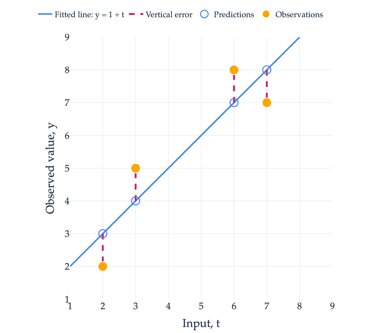
For our four points (3,5)(3,5), (2,2)(2,2), (7,7)(7,7), and (6,8)(6,8), the model is y=c+mty=c+mt, with

A=[13121716],bāƒ—=[5278].A=\begin{bmatrix}1&3\\1&2\\1&7\\1&6\end{bmatrix},\qquad \vec b=\begin{bmatrix}5\\2\\7\\8\end{bmatrix}.

Calculate the products:

ATA=[11113276][13121716]=[4181898],A^TA =\begin{bmatrix}1&1&1&1\\3&2&7&6\end{bmatrix} \begin{bmatrix}1&3\\1&2\\1&7\\1&6\end{bmatrix} =\begin{bmatrix}4&18\\18&98\end{bmatrix},
ATbāƒ—=[11113276][5278]=[22116].A^T\vec b =\begin{bmatrix}1&1&1&1\\3&2&7&6\end{bmatrix} \begin{bmatrix}5\\2\\7\\8\end{bmatrix} =\begin{bmatrix}22\\116\end{bmatrix}.

The normal equations for xāƒ—āˆ—=[cāˆ—māˆ—]\vec x^*=\begin{bmatrix}c^*\\m^*\end{bmatrix} are therefore

4cāˆ—+18māˆ—=22,18cāˆ—+98māˆ—=116.\begin{aligned} 4c^*+18m^*&=22,\\ 18c^*+98m^*&=116. \end{aligned}

Twice the second equation minus nine times the first gives 34māˆ—=3434m^*=34, so māˆ—=1m^*=1. Then the first equation gives cāˆ—=1c^*=1, so

xāƒ—āˆ—=[11],y=1+t.\boxed{\vec x^*=\begin{bmatrix}1\\1\end{bmatrix},\qquad y=1+t.}

The predictions and error vector are

pāƒ—=Axāƒ—āˆ—=[4387],rāƒ—=bāƒ—āˆ’pāƒ—=[1āˆ’1āˆ’11].\vec p=A\vec x^*=\begin{bmatrix}4\\3\\8\\7\end{bmatrix},\qquad \vec r=\vec b-\vec p=\begin{bmatrix}1\\-1\\-1\\1\end{bmatrix}.

Check the error vector’s dot products with the two columns:

ATrāƒ—=[1āˆ’1āˆ’1+13āˆ’2āˆ’7+6]=[00].A^T\vec r=\begin{bmatrix}1-1-1+1\\3-2-7+6\end{bmatrix} =\begin{bmatrix}0\\0\end{bmatrix}.

The error vector is perpendicular to the column space, confirming that we found the closest output. The minimum squared error length is

∄rāƒ—āˆ„2=12+(āˆ’1)2+(āˆ’1)2+12=4.\|\vec r\|^2=1^2+(-1)^2+(-1)^2+1^2=4.

The original equations remain inconsistent, but we now know exactly how close their left-hand sides can get to their right-hand sides.

<IPython.core.display.Image object>

Exploring squared error

Each choice of intercept cc and slope mm gives a line on the left. The dashed segments show the vertical errors. On the right, the pink dot records the same choice of cc and mm, with height ∄rāƒ—āˆ„2\|\vec r\|^2, the sum of squared errors.

Try c=0c=0 and m=1m=1, then c=2c=2 and m=1m=1. Both choices give squared error 8. What happens if you set c=1c=1 and keep m=1m=1? Use the sliders to see how changing either coefficient moves the dot on the surface.

The mean squared error is the sum of squared errors divided by the number of observations, here 4. This rescales the height of the surface, so both objectives reach their minimum at the same line. The normal equation tells us where that minimum is without having to search with the sliders.
Loading...